library(tidyverse)2 Demographics
The demographics form captures the descriptive and background characteristics of each A2CPS participant: age, sex, gender identity, race and ethnicity, education, employment, marital status, household income, disability status, dominant hand, height and weight, pain duration, and a few COVID-related items. Almost every A2CPS analysis draws on these fields so demographics is often the first modality a project touches. Participants also belong to one of two surgical cohorts (knee arthroplasty and thoracic surgery), and since these cohorts differ systematically in age and body composition, the demographic variables matter when we interpret cohort comparisons.
Many fields are coded categorical values (for example, sex is 1 = Male, 2 = Female), with the codes defined in the accompanying data dictionary. In addition to the raw fields, the cleaning workflow computes a validated body mass index (BMI) from height and weight, and attaches a set of data-quality flags that mark implausible or logically inconsistent values so that we can decide how to handle them.
2.1 Starting Project
2.1.1 Locate Data
Where are the relevant files?
$ /corral-secure/projects/A2CPS/products/consortium-data/pre-surgery-release-2-1-0/demographics/reformattedThe reformatted data are in a single file, reformatted_demo.csv (one row per participant), together with demo_dict_updated.csv. The dictionary is essential here, since it lists the coded values for every categorical field (sex, genident, ethnic, edulevel, empstat, maristat, incmlvl, and so on) alongside the fields added during cleaning.
2.1.2 Extract Data
The file is a plain CSV, and here we use the tidyverse.
demo <- read_csv("data/pre-surgery/demographics/reformatted/reformatted_demo.csv")Since the categorical fields are stored as numeric codes, using the data dictionary as a reference is highly recommended (demo_dict_updated.csv).
demo_dict <- read_csv("data/pre-surgery/demographics/reformatted/demo_dict_updated.csv")

demo_dict |>
  filter(field_name == "sex") |>
select(field_name, select_choices_or_calculations)| field_name | select_choices_or_calculations |
|---|---|
| sex | 1, Male | 2, Female | 3, Unknown | 4, Intersex |
Next, a quick look at the continuous fields and the cohort label:
demo |>
  select(record_id, cohort, age, sex, bmi_kg_m2, paindur) |>
head()| record_id | cohort | age | sex | bmi_kg_m2 | paindur |
|---|---|---|---|---|---|
| 10001 | TKA | 68 | 2 | 32.99943 | 2 |
| 10003 | TKA | 73 | 2 | 22.13865 | 12 |
| 10004 | TKA | 64 | 2 | 35.17960 | 9 |
| 10005 | TKA | 58 | 1 | 28.75630 | 144 |
| 10006 | TKA | 55 | 1 | 44.04175 | 12 |
| 10007 | TKA | 63 | NA | 35.95317 | 6 |
glimpse() confirms the data types. Note that the coded categoricals come in as numbers, so we recode them to labelled factors before summarizing or plotting.
demo |>
  select(record_id, cohort, age, sex, edulevel, bmi_kg_m2, paindur) |>
  glimpse()
Rows: 1,933
Columns: 7
$ record_id <dbl> 10001, 10003, 10004, 10005, 10006, 10007, 10008, 10010, 1001…
$ cohort <chr> "TKA", "TKA", "TKA", "TKA", "TKA", "TKA", "TKA", "TKA", "TKA…
$ age <dbl> 68, 73, 64, 58, 55, 63, 73, 64, 54, 53, 71, 45, 65, 59, 56, …
$ sex <dbl> 2, 2, 2, 1, 1, NA, 2, 1, 1, 1, 2, NA, 2, 2, NA, 1, 2, 1, 2, …
$ edulevel <dbl> 5, 5, 4, 6, 4, 5, 3, 4, 5, 4, 6, 6, 4, 6, 3, 3, 5, 6, 6, 5, …
$ bmi_kg_m2 <dbl> 32.99943, 22.13865, 35.17960, 28.75630, 44.04175, 35.95317, …
$ paindur <dbl> 2, 12, 9, 144, 12, 6, 660, 64, 84, 192, 60, 60, 96, 36, 36, …2.1.3 Data Quality
The reformatted file has already been cleaned. It keeps the implausible values and flags them instead of dropping them, which lets the end user decide how to handle each flagged value. The flag columns are:
bmi_measurement_issueandheight_weight_check: these mark BMI values built from missing or implausible height and weight. Most records are"Valid Range", but a small number are flagged. The rawbmi_kg_m2column still contains extreme values (as low as 2 and as high as 64).paindur_outlier_flag: flags pain-duration values that are zero or negative (~200 records), extreme statistical outliers (~80), or logically impossible (pain lasting longer than the participant has been alive).age_outlier_flagandage_pain_logic_error: these mark missing ages and cases where the reported pain duration exceeds the participant’s total months of life.covid_logic_error: flags internally inconsistent COVID responses (e.g., a “No” with a follow-up detail still answered).dom_hand_statusandincmlvl_clean: cleaned, human-readable versions of dominant hand and income level.
It helps to tally a flag first and see how many records get affected:
demo |>
count(bmi_measurement_issue)| bmi_measurement_issue | n |
|---|---|
| Check Raw Data: Flag: Height Ft Implausible | 3 |
| Check Raw Data: Flag: Height Inches Implausible | 2 |
| Check Raw Data: Flag: Weight Implausible | 1 |
| Check Raw Data: Missing Raw Data | 68 |
| Flag: Implausibly High BMI | 3 |
| Valid Range | 1856 |
2.1.4 Cross-Modality Links
Every file includes record_id and guid, which uniquely identify a participant and let us link demographics to other A2CPS modalities. Since demographics is almost always used as covariates for another modality, the typical join attaches these background fields to a primary analysis table:
inner_join(other_modality, demo, by = intersect(names(other_modality), names(demo)))2.2 Exploratory data analysis
Since the two surgical cohorts are recruited separately, a useful way to get oriented is to compare their basic demographics, because the differences here shape the interpretation of cohort comparisons. We look at age and BMI, and we use the quality flags to keep only the analysis-ready BMI values.
demo_clean <- demo |>
  mutate(
    cohort = factor(cohort),
    bmi = if_else(bmi_measurement_issue == "Valid Range", bmi_kg_m2, NA_real_)
  )

demo_clean |>
  group_by(cohort) |>
  summarise(
    n          = n(),
    age_mean   = mean(age, na.rm = TRUE),
    bmi_mean   = mean(bmi, na.rm = TRUE)
)| cohort | n | age_mean | bmi_mean |
|---|---|---|---|
| Thoracic | 527 | 60.24658 | 29.37161 |
| TKA | 1406 | 65.31789 | 31.34604 |
As expected, the knee (TKA) cohort is both older and heavier on average (age ≈ 65 vs. 60; BMI ≈ 31 vs. 29), which fits the usual clinical profile of knee-arthroplasty candidates. Let’s look at the full distributions with side-by-side boxplots.
ggplot(demo_clean, aes(x = cohort, y = age, fill = cohort)) +
  geom_boxplot(show.legend = FALSE) +
  labs(title = "Age by cohort", x = NULL, y = "Age (years)") +
  theme_minimal()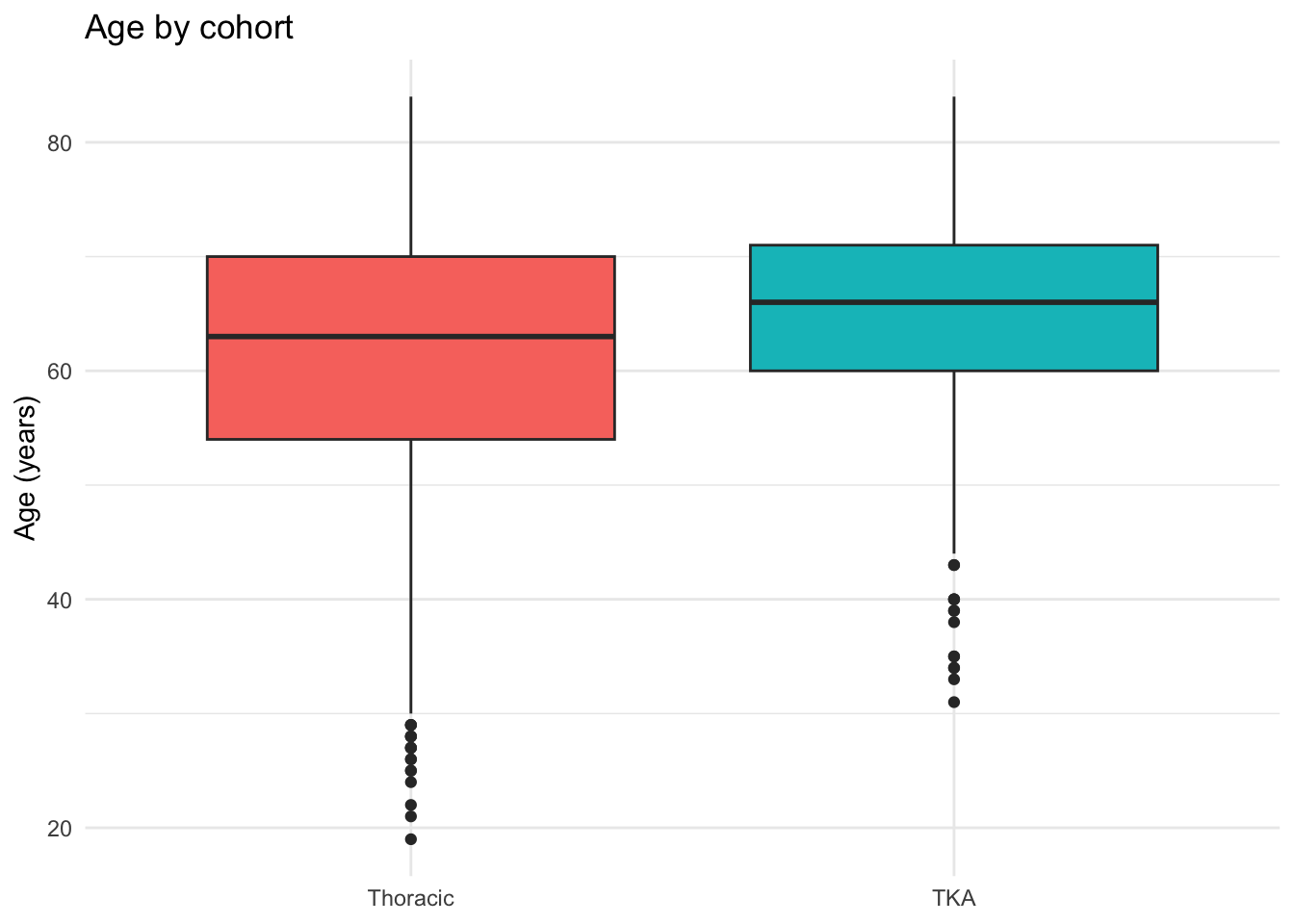
demo_clean |>
  filter(!is.na(bmi)) |>
  ggplot(aes(x = cohort, y = bmi, fill = cohort)) +
  geom_boxplot(show.legend = FALSE) +
  labs(title = "BMI by cohort (quality-flagged values removed)",
       x = NULL, y = expression(BMI~(kg/m^2))) +
  theme_minimal()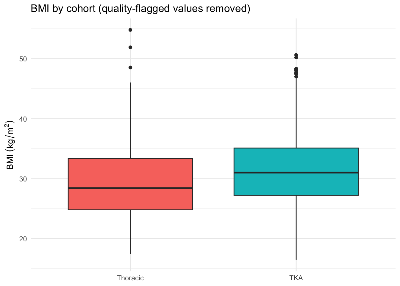
The takeaway for planning is that the cohorts are not demographically interchangeable, so age and BMI are natural covariates to consider whenever we pool or compare them.
2.3 Considerations While Working on the Project
2.3.1 Data Generation
Demographic information is self-reported by participants at baseline through REDCap, following the A2CPS Manual of Procedures. Height and weight are used to derive BMI. The steps that turn the REDCap export into the reformatted file (recoding, BMI computation, and the plausibility and logic checks that populate the flag columns) are documented in the cleaning workflow that comes with the release.
2.3.2 Other
- Coded fields. Most categorical fields are stored as numbers, and the coding differs from field to field, so it helps keep
demo_dict_updated.csvhandy. - Sparse Data. A few fields have very sparse levels (for example, the handful of Unknown and Intersex responses in
sex), which can make those subgroups unstable. - Self-report. These fields are all self-reported at baseline, so the usual survey caveats apply, such as some missingness, rounding in height, weight, and pain duration, and bias in items like income.
- Quality control. The cleaning pipeline has been reviewed, and the flag columns serve as its record, showing which values were questioned and why. The checks can be re-derived from the accompanying cleaning workflow.
2.3.3 Citations
In publications or presentations including data from A2CPS, please include the following statement as attribution:
Data were provided (in part) by the A2CPS Consortium funded by the National Institutes of Health (NIH) Common Fund, which is managed by the Office of the Director (OD)/Office of Strategic Coordination (OSC). Consortium components and their associated funding sources include Clinical Coordinating Center (U24NS112873), Data Integration and Resource Center (U54DA049110), Omics Data Generation Centers (U54DA049116, U54DA049115, U54DA049113), Multi-site Clinical Center 1 (MCC1) (UM1NS112874), and Multi-site Clinical Center 2 (MCC2) (UM1NS118922).
Note
Berardi, G., Frey-Law, L., Sluka, K. A., Bayman, E. O., Coffey, C. S., Ecklund, D., Vance, C. G. T., Dailey, D. L., Burns, J., Buvanendran, A., McCarthy, R. J., Jacobs, J., Zhou, X. J., Wixson, R., Balach, T., Brummett, C. M., Clauw, D., Colquhoun, D., Harte, S. E., … Wandner, L. D. (2022). Multi-site observational study to assess biomarkers for susceptibility or resilience to chronic pain: The acute to chronic pain signatures (A2CPS) study protocol. Frontiers in Medicine, 9. https://doi.org/10.3389/fmed.2022.849214
Sluka, K. A., Wager, T. D., Sutherland, S. P., Labosky, P. A., Balach, T., Bayman, E. O., Berardi, G., Brummett, C. M., Burns, J., Buvanendran, A., et al. (2023). Predicting chronic postsurgical pain: Current evidence and a novel program to develop predictive biomarker signatures. Pain, 164(9), 1912–1926. https://doi.org/10.1097/j.pain.0000000000002938