library(fs)
library(ggplot2)
library(readr)
library(tidyr)16 Primary DWI Biomarker
In Chapter 15, we covered the outputs of BedpostX, which is a method for modeling how water diffuses in each voxel and estimating their implied fiber orientation distributions. The outputs of BedpostX were used as the inputs for probabilistic tractography—a technique that repeatedly samples from these distributions to build “streamlines” representing probable neural tracts. By modeling the uncertainty of fiber orientations, probabilistic tractography is uniquely capable of reconstructing complex, long-distance networks, including the corticolimbic network.
Specifically, this kit describes the derivatives produced while extracting one of the primary A2CPS biomarkers. This biomarker is based on a finding reported by Vachon-Presseau et al. (2016): as compared with patients whose subacute back pain recovered, those whose pain persisted exhibited higher connectivity at baseline within a corticolimbic subnetwork involving the amygdala, nucleus accumbens, and the dorsal medial prefrontal cortex (Am-NAc-mPFC).
16.1 Starting Project
16.1.1 Locate Data
On TACC, the data are stored underneath the releases. For example, data release v2.1.0 is underneath
/corral-secure/projects/A2CPS/products/consortium-data/pre-surgery-release-2-1-0Paths in this kit are written relative to that release folder, so the neuroimaging data are underneath mris.
The derivatives for this biomarker are a collection of three kinds of outputs:
$ ls mris/derivatives/dwi_biomarker1/
move_masks  networks  probtrackx
Each of these are organizing in a “BIDS-ish” manner.
$ tree mris/derivatives/dwi_biomarker1/move_masks/sub-10003
mris/derivatives/dwi_biomarker1/move_masks/sub-10003
└── ses-V1
    └── dwi
        ├── sub-10003_ses-V1_masks
        ├── sub-10003_ses-V1_space-dwi_desc-modules_dseg.nii.gz
        ├── sub-10003_ses-V1_space-dwifslstd_desc-module0_dseg.nii.gz
        ├── sub-10003_ses-V1_space-dwifslstd_desc-module1_dseg.nii.gz
        └── sub-10003_ses-V1_space-dwifslstd_desc-module2_dseg.nii.gz
2 directories, 5 files

$ tree mris/derivatives/dwi_biomarker1/networks/sub-10003
mris/derivatives/dwi_biomarker1/networks/sub-10003
└── ses-V1
    └── dwi
        └── network_summaries.tsv
2 directories, 1 file

$ tree mris/derivatives/dwi_biomarker1/probtrackx/sub-10003
mris/derivatives/dwi_biomarker1/probtrackx/sub-10003
└── ses-V1
    └── dwi
        ├── coords_for_fdt_matrix1
        ├── fdt_matrix1.dot.gz
        ├── fdt_paths.nii.gz
        ├── probtrackx.log
        └── waytotal
2 directories, 5 files- move_masks
- The biomarker is calculated in the native dwi space. These files contain information about
*space-dwi_desc-modules_dseg.nii.gz: the relevant masks in participant-native dwi space. All three subnetworks are contained as non-overlapping clusters.*space-dwifslstd_desc-module*_dseg.nii.gz: Binary mask files for each of the three subnetworks.*masksa text file pointing to each of the binary mask files that is used as input for theprobtrackxstep.
- The biomarker is calculated in the native dwi space. These files contain information about
- probtrackx
- Results from probabilistic tract tracing (with ProbtrackX).
- networks
- Tabular information summarizing connectivity within the networks.
Most users will be interested in the tabular information. A data dictionary is available at the top-level of the network folder (derivatives/dwi_biomarker1/network_summaries.json). Note that we use the terms “subnetwork” and “module” interchangeably.
{
    "Deg_mean": {
        "LongName": "Mean Degree",
        "Description": "Average nodal degree within module (after thresholding network to 10% density)",
        "TermURL": "https://networkx.org/documentation/stable/reference/classes/generated/networkx.Graph.degree.html"
    },
    "Density": {
        "LongName": "Density",
        "Description": "Density of the module (after thresholding network to 10% density)",
        "TermURL": "https://networkx.org/documentation/stable/reference/generated/networkx.classes.function.density.html"
    },
    "WM_connections": {
        "LongName": "White Matter Connections",
        "Description": "A summary of the total connections in the network: sum(Degs) / (nvox * (nvox - 1) / 2)"
    },
    "ModuleNumber": {
        "LongName": "Module Number",
        "Description": "Index of the network module"
    },
    "ModuleName": {
        "LongName": "Module Name",
        "Description": "Name of the module from the reference (https://doi.org/10.1093/brain/aww100)",
        "Levels": {
            "mPFCventral-amyg": "ventral medial PFC–amygdala",
            "OFC-amyg-hipp": "orbitofrontal cortex–amygdala–hippocampus",
            "mPFCdorsal-amyg-NAc": "dorsal medial PFC–amygdala–nucleus accumbens",
            "WholeNetwork": "Full network (not a module)"
        }
    },
    "IsBiomarker": {
        "LongName": "Biomarker Indicator",
        "Description": "Boolean indicating whether this module is a primary biomarker for A2CSP"
    },
    "sub": {
        "LongName": "Subject",
        "Description": "Study Participant, BIDS Subject ID",
        "TermURL": "https://bids-specification.readthedocs.io/en/v1.9.0/appendices/entities.html#sub"
    },
    "ses": {
        "LongName": "Session",
        "Description": "Visit, Protocol, BIDS Session ID",
        "Levels": {
            "V1": "baseline_visit",
            "V3": "3mo_postop"
        },
        "TermURL": "https://bids-specification.readthedocs.io/en/v1.9.0/appendices/entities.html#ses"
    }
}
16.1.2 Extract Data
The tables always have the same schema and so can be loaded together using standard tools.
networks <- read_tsv(dir_ls(
  "data/pre-surgery/mris/derivatives/dwi_biomarker1/networks",
  glob = "*tsv",
  recurse = TRUE
))

head(networks)| Deg_mean | Density | WM_connections | ModuleNumber | ModuleName | IsBiomarker | sub | ses |
|---|---|---|---|---|---|---|---|
| 434.1132 | 0.0811123 | 0.1622247 | 0 | mPFCventral-amyg | FALSE | 10008 | V1 |
| 310.6833 | 0.0960085 | 0.1920169 | 1 | OFC-amyg-hipp | FALSE | 10008 | V1 |
| 271.9534 | 0.1441194 | 0.2882389 | 2 | mPFCdorsal-amyg-NAc | TRUE | 10008 | V1 |
| 664.1328 | 0.0633836 | 0.1267671 | NA | WholeNetwork | FALSE | 10008 | V1 |
| 170.8519 | 0.0229825 | 0.0459650 | 0 | mPFCventral-amyg | FALSE | 10010 | V1 |
| 114.8354 | 0.0291683 | 0.0583365 | 1 | OFC-amyg-hipp | FALSE | 10010 | V1 |
For understanding these, it may help to plot all available metrics.
networks |>
  pivot_longer(c(Deg_mean, Density, WM_connections), names_to = "metric") |>
  ggplot(aes(y = ModuleName, x = value)) +
  facet_wrap(~metric, scales = "free_x") +
  geom_boxplot(outliers = FALSE) +
  # seeded so the figure is reproducible across renders
  geom_point(alpha = 0.2, position = position_jitter(seed = 1))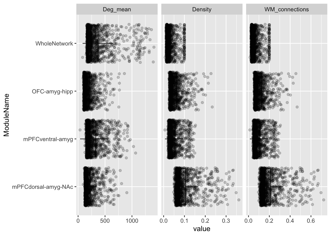
In Figure 16.1, we can see that the thresholding did not affect most connectivity matrices: the density of the whole network was already below 10%. Nevertheless, there is variability in the subnetworks that may have predictive value.
16.2 Considerations While Working on the Project
16.2.1 Data Generation
The pipeline for this connectivity biomarker was extracted by first passing outputs of BEDPOSTX to FSL’s probabilistic tractography routine PROBTRACKX2. When conducting the tracking, the following options were used: a loop check, a one-way condition, a curvature threshold of 0.2, 2000 steps, a step length of 0.5, 5000 samples, a 0.01 volume fraction threshold for consideration of subsidiary fiber orientations, a distance threshold of 0, no random sampling around the voxel, modified Euler streamlining, and correction of path distributions for path length. Note that the probtrackx command is present in a log file for each participant (e.g., derivatives/dwi_biomarker1/probtrackx/sub-10003/probtrackx.log).
As a seed for probabilistic tractography, we used a voxel-wise corticolimbic mask from Vachon-Presseau et al. (2016). This mask comprised three subnetworks: the Am-NAc-mPFC, a ventral mPFC-Amygdala network, and one involving the amygdala, hippocampus, and orbitofrontal cortex. The resulting connectivity matrix was symmetrized and binarized (thresholded to a density of 10%). The final biomarker was the total degree of the nodes within the subnetwork divided by the maximum possible number of connections in the subnetwork. This connectivity analysis was performed in each subject’s native space (1.7 mm3); the corticolimbic mask was transformed into native space using the warps estimated by QSIPrep during preprocessing, with ANTs (nearest-neighbor interpolation).
16.2.2 Interpretation of “Streamlines”
The information provided by probabilistic tracktography is often misrepresented. If you are brand new to the subject, the official FSL tutorial on PROBTRACKX is recommended. In particular, keep in mind is that, although we often want to know information about the “strength” or “integrity” of connections, ProbtrackX only provides information about whether a connection between two regions is likely; more streamlines correspond to higher chances of there being a connection, and not anything about the quality or size of those connections. There is almost certainly a relationship between whether ProbtrackX determines a connection to be likely and the strength of a connection, with strength meaning something like the capacity for information flow, or, more concretely, the number of dendrites comprising a track. But the nature of that relationship is unknown, and caution should be exercised when describing these outputs.
16.2.3 Calculating Additional Metrics
In some analyses, it may be interesting to go back to the connectivity graphs as output by ProbtrackX (e.g., to explore alternative thresholds). In that case, you would need to start with the files in derivatives/dwi_biomarker1/probtrackx. Example code for working with those files is available here. The key point is that ProbtrackX stores the connectivity outputs in an asymmetric Coordinate List format (the asymmetry implies that there are entries for both source -> target and target -> source, even though the connections themselves are undirected).
16.2.4 Variability Across Scanners
Many MRI biomarkers exhibit variability across the scanners, which may confound some analyses. For an up-to-date assessment of the issue and overview of current thinking, please see Appendix D.
16.2.5 Data Quality
As with any MRI derivative, all pipeline derivatives have been included. This means that products were included regardless of their quality, and so some products may have been generated from images that are known to have poor quality—rated “red”, or incomparable. For details on the ratings and how to exclude them, see Appendix A. Additionally, extensive QC has not yet been performed on the derivatives themselves, and so there may be cases where pipelines produced atypical outputs. For an overview of planned checks, see Confluence.
16.2.6 Data Generation
These outputs were generated by the dwi_biomarker1_app.
16.2.7 Citations
If you use these products in your analyses, please cite the relevant papers from FSL. Additionally, please cite the source of this biomarker (Vachon-Presseau et al., 2016).
Vachon-Presseau, E., Tétreault, P., Petre, B., Huang, L., Berger, S. E., Torbey, S., Baria, A. T., Mansour, A. R., Hashmi, J. A., Griffith, J. W., et al. (2016). Corticolimbic anatomical characteristics predetermine risk for chronic pain. Brain, 139(7), 1958–1970. https://doi.org/10.1093/brain/aww100
In publications or presentations including data from A2CPS, please include the following statement as attribution:
Data were provided (in part) by the A2CPS Consortium funded by the National Institutes of Health (NIH) Common Fund, which is managed by the Office of the Director (OD)/Office of Strategic Coordination (OSC). Consortium components and their associated funding sources include Clinical Coordinating Center (U24NS112873), Data Integration and Resource Center (U54DA049110), Omics Data Generation Centers (U54DA049116, U54DA049115, U54DA049113), Multi-site Clinical Center 1 (MCC1) (UM1NS112874), and Multi-site Clinical Center 2 (MCC2) (UM1NS118922).
Note
Berardi, G., Frey-Law, L., Sluka, K. A., Bayman, E. O., Coffey, C. S., Ecklund, D., Vance, C. G. T., Dailey, D. L., Burns, J., Buvanendran, A., McCarthy, R. J., Jacobs, J., Zhou, X. J., Wixson, R., Balach, T., Brummett, C. M., Clauw, D., Colquhoun, D., Harte, S. E., … Wandner, L. D. (2022). Multi-site observational study to assess biomarkers for susceptibility or resilience to chronic pain: The acute to chronic pain signatures (A2CPS) study protocol. Frontiers in Medicine, 9. https://doi.org/10.3389/fmed.2022.849214
Sluka, K. A., Wager, T. D., Sutherland, S. P., Labosky, P. A., Balach, T., Bayman, E. O., Berardi, G., Brummett, C. M., Burns, J., Buvanendran, A., et al. (2023). Predicting chronic postsurgical pain: Current evidence and a novel program to develop predictive biomarker signatures. Pain, 164(9), 1912–1926. https://doi.org/10.1097/j.pain.0000000000002938
Sadil, P., Arfanakis, K., Bhuiyan, E. H., Caffo, B., Calhoun, V. D., Clauw, D. J., DeLano, M. C., Ford, J. C., Gattu, R., Guo, X., Harris, R. E., Ichesco, E., Johnson, M. A., Jung, H., Kahn, A. B., Kaplan, C. M., Leloudas, N., Lindquist, M. A., Luo, Q., … Chronic Pain Signatures Consortium, T. A. to. (2024). Image processing in the acute to chronic pain signatures (A2CPS) project. bioRxiv. https://doi.org/10.1101/2024.12.19.627509
When using neuroimaging derivatives, please also cite Sadil et al. (2024).