[[20]{.chapter-number}  [MRIQC]{.chapter-title}]{#sec-mriqc .quarto-section-identifier}

20 MRIQC

library(dplyr)
library(duckplyr)
library(fs)
library(ggplot2)
library(readr)
library(scattermore)

Rigorous quality control (QC) is absolutely essential in neuroimaging. Artifacts like participant head motion, scanner thermal noise, or radio-frequency (RF) coil failures can dramatically compromise the integrity of the data and introduce severe confounds into downstream analyses. To automatically calculate a suite of standardized image quality metrics, the A2CPS project uses the widely adopted MRI Quality Control (MRIQC) pipeline (Esteban et al., 2017).

Part of the A2CPS MRI quality control procedure Section 5.2.1 relies directly on these MRIQC metrics. However, MRIQC provides several additional metrics beyond the subset formally used by A2CPS. This kit reviews those metrics and demonstrates how you can benchmark A2CPS data against the hundreds of thousands of scans available in the public MRIQC database.

20.1 Starting Project

20.1.1 Locate Data

On TACC, the data are stored underneath the releases. For example, data release v2.1.0 is underneath

/corral-secure/projects/A2CPS/products/consortium-data/pre-surgery-release-2-1-0

Paths in this kit are written relative to that release folder, so the neuroimaging data are underneath mris.

The MRIQC metrics are underneath derivatives/mriqc.

20.1.2 Extract Data

The A2CPS pipeline produces a standard set of MRIQC outputs, including both participant- and group-level results. For a detailed explanation of the outputs, please see the official MRIQC documentation. At a high-level, the outputs include:

participant-level metrics: underneath sub-[record_id]/ses-[protocol_id]/{anat,func,dwi}
participant-level reports: html documents that display participant-level figures related to data quality and MRIQC preprocessing
group-level results: files with the prefix group_ that collate the participant-level results

$ ls mris/derivatives/mriqc | head
group_bold.html
group_bold.tsv
group_dwi.html
group_dwi.tsv
group_T1w.html
group_T1w.tsv
sub-10003
sub-10003_ses-V1_dwi.html
sub-10003_ses-V1_T1w.html
sub-10003_ses-V1_task-cuff_run-01_bold.html

For example, here are all of the metrics available for the functional data.

group_bold <- read_tsv("data/pre-surgery/mris/derivatives/mriqc/group_bold.tsv")
group_bold |> head()

fd_num	dvars_vstd	aqi	summary_bg_mad	size_z	summary_bg_p95	summary_fg_stdv	summary_fg_n	size_x	dvars_std	fwhm_y	fwhm_z	gcor	spacing_tr	spacing_y	spacing_z	gsr_x	gsr_y	dummy_trs	summary_fg_k	summary_bg_median	efc	fwhm_x	spacing_x	fwhm_avg	summary_bg_stdv	tsnr	summary_fg_p95	fber	dvars_nstd	summary_bg_k	summary_fg_mad	fd_mean	size_y	summary_bg_n	aor	size_t	summary_fg_median	summary_fg_p05	summary_bg_mean	fd_perc	summary_fg_mean	snr	bids_name
29	0.9178377	0.0248978	19.2671	60	503	438.5144	91243	90	1.003084	2.607900	2.814183	0.0017190	0.8000000	2.40000	2.4	0.0069208	-0.0092690	7	3.9317	13	0.4557	3.059612	2.40000	2.827232	241.9392	31.13016	1949	7617.007	34.46851	46.5662	309.1644	0.1216549	90	394757	0.0012493	443	1099	512	86.1477	6.546275	1153.679	2.506175	sub-11129_ses-V1_task-rest_run-01_bold
336	0.9843680	0.0460471	20.4753	60	198	387.1901	107092	90	1.117544	2.692258	2.942400	0.0053764	0.8000000	2.40000	2.4	0.0152008	0.0259423	7	1.2213	14	0.4640	2.888658	2.40000	2.841105	114.1635	20.18094	1521	4644.043	67.01637	79.5274	290.6688	0.5365611	90	378908	0.0057026	443	929	155	47.9287	75.846501	906.543	2.399327	sub-25195_ses-V3_task-rest_run-01_bold
332	0.9640853	0.0351266	240.1816	54	5383	11654.6264	98367	96	1.094660	2.596908	2.434958	0.0030409	0.7999997	2.21875	2.4	-0.0112133	0.0173554	3	1.1931	162	0.4466	2.684061	2.21875	2.571976	2865.4246	27.58617	55006	58541.832	53.59101	119.5800	7726.8189	0.3381134	96	399297	0.0005851	447	39116	12403	1440.0459	74.272931	37912.920	3.356247	sub-10804_ses-V1_task-cuff_run-01_bold
242	0.9842039	0.0064706	28.1694	60	506	717.7262	98733	90	1.127007	3.502229	3.400621	0.0164867	0.8000000	2.40000	2.4	-0.0071657	0.0262937	5	0.6940	19	0.4565	3.318537	2.40000	3.407129	221.5842	44.80010	2917	6779.601	37.33743	40.1238	619.0548	0.2159795	90	387267	0.0005034	445	1579	428	97.1042	54.382022	1631.007	2.199992	sub-20136_ses-V1_task-rest_run-02_bold
433	1.0132514	0.0468254	65.2345	54	3300	5080.0158	104331	96	1.176027	2.804890	2.584008	0.0075407	0.7999997	2.21875	2.4	-0.0077151	0.0393644	3	1.5830	44	0.4626	2.765255	2.21875	2.718051	1691.5409	23.29130	25293	173228.391	78.35565	57.2196	3681.2955	0.8988191	96	393333	0.0033332	447	18209	7445	754.2399	96.868009	17816.636	3.584420	sub-10067_ses-V3_task-cuff_run-02_bold
122	0.9972909	0.0133522	20.5917	60	270	417.7710	100017	90	1.055689	2.430671	2.566229	0.0041807	0.8000000	2.40000	2.4	0.0104461	0.0184142	9	2.8760	14	0.4586	2.631387	2.40000	2.542762	141.5572	31.36398	1800	5164.810	35.86010	49.7461	306.7541	0.1455054	90	385983	0.0025216	441	1005	397	57.6900	27.664399	1050.347	2.405612	sub-10514_ses-V3_task-cuff_run-02_bold

For a detailed description of these metrics, please see the official MRIQC documentation.

20.1.3 Comparison with Reference Distributions

One strength of MRIQC is that the pipeline automatically stores the metrics in a centralized database. The centralized database is available via the MRIQC Web API. An example of interacting with the API can be found in https://github.com/psadil/mriqc-export. In this kit, the metrics have already been downloaded and stored in a set parquet files. Let’s use that reference set to rate A2CPS. One of the most important determiners of quality is motion, so let’s focus on the average Framewise Displacement.

all_bold <- read_parquet_duckdb(dir_ls(
  "data/mriqcwebapi/bold",
  recurse = TRUE,
  glob = "*parquet"
)) |>
  select(`_id`, fd_mean) |>
  collect()

nrow(all_bold)

[1] 1245400

Loading them, we see that there are over 1 million entries in the database.

Let’s create a simple scatter plot to compare motion in A2CPS against motion in the MRIQC database. Note that because there are so many points to display, we’re using the package scattermore.

bind_rows(list(a2cps = group_bold, mriqc = all_bold), .id = "source") |>
  ggplot(aes(x = source, y = fd_mean)) +
  geom_violin() +
  geom_scattermore(position = position_jitter(height = 0, seed = 1)) +
  coord_cartesian(ylim = c(0, 5))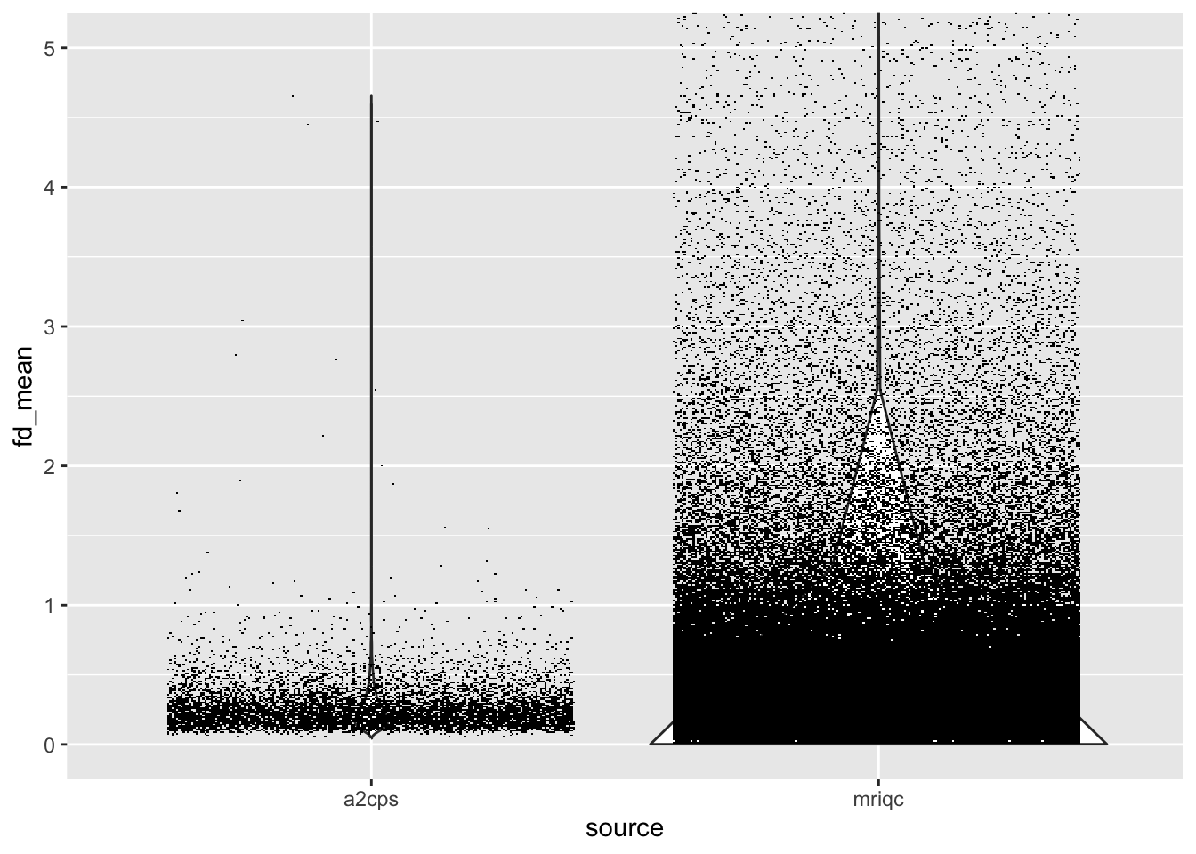

Quantitatively, the dataset is in the upper quantiles of motion, which is to be expected given the study population (i.e. patients suffering from chronic pain and discomfort).

empirical_motion_cdf <- ecdf(all_bold$fd_mean)

group_bold |>
  mutate(fd_quantile = empirical_motion_cdf(fd_mean)) |>
  ggplot(aes(x = fd_quantile)) +
  geom_histogram()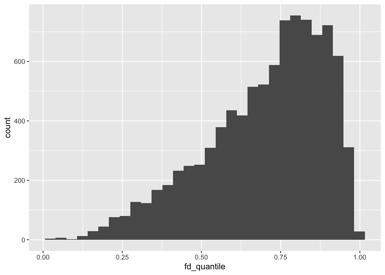

Quantiles of Mean Framewise Displacement in A2CPS. The quantiles are calculated from an empirical CDF derived from the MRIQC reference database.

20.2 Considerations While Working on the Project

20.2.1 Framewise Displacement and A2CPS

A key element of the A2CPS Quality Ratings for raw data is based on Framewise Displacement. Although MRIQC provides a measurement of framewise displacement, it is not the one that is entered into the rating. Instead, A2CPS uses the estimate of motion from fMRIPrep, what it refers to as rmsd, also referred to as FD_Jenk, in reference to the method as described in Jenkinson et al. (2002). The measure of motion provided by MRIQC is sometimes referred to as FD_Power (e.g., Parkes et al. (2018)), referring to Power et al. (2012). FD_Power measures the distance travelled by a point on the edge of a sphere between frames (usually using a sphere of 50 mm), whereas FD_Jenk measures the average distance traveled by the entire sphere (usually using a sphere of 80 mm). The two measures are often almost perfectly correlated, but FD_Power tends to be about 1.7x as high as FD_Jenk.

Jenkinson, M., Bannister, P., Brady, M., & Smith, S. (2002). Improved optimization for the robust and accurate linear registration and motion correction of brain images. Neuroimage, 17(2), 825–841. https://doi.org/10.1006/nimg.2002.1132

Parkes, L., Fulcher, B., Yücel, M., & Fornito, A. (2018). An evaluation of the efficacy, reliability, and sensitivity of motion correction strategies for resting-state functional MRI. Neuroimage, 171, 415–436. https://doi.org/10.1016/j.neuroimage.2017.12.073

Power, J. D., Barnes, K. A., Snyder, A. Z., Schlaggar, B. L., & Petersen, S. E. (2012). Spurious but systematic correlations in functional connectivity MRI networks arise from subject motion. Neuroimage, 59(3), 2142–2154. https://doi.org/10.1016/j.neuroimage.2011.10.018

20.2.2 MRIQC Versions

Please be aware that, across versions of MRIQC, the manner in which MRIQC calculates metrics has changed. These changes can lead to substantial differences in the distribution of metrics. For one set of examples, please see this GitHub issue.

20.2.3 Variability Across Scanners

Many of these metrics exhibit substantial variability across the scanners, which may confound some analyses. For example, the scanner “NS” (serial number: 70032) has the “Prescan Normalization” feature turned off, which produces substantial intensity inhomogeneity in the images. This inhomogeneity is very noticeable in the images, resulting in much voxels near the edge of the field-of-view being much brighter than voxels in the center of the field-of-view. Unfortunately, this spatial pattern confounds one of the metrics produced by MRIQC that is designed to estimate ghosting: the “Ghost-to-Signal” Ratio. That is, the values for this ratio suggest that the NS scanner suffers from substantial ghosting, but those values are instead driven primarily by intensity inhomogeneity.

As another example, the scanner UC (serial number: 71399) is unique in that the structural images were collected with “Image Domain Parallel Imaging”. This form of parallel imaging causes a near total suppression of the background signal (that is, most background voxels have intensity 0). Several of the MRIQC metrics incorporate the background signal, and so this noise suppression causes those metrics to have a fundamentally different scaling as compared to metrics calculated on images without that suppression. Consider the “Dietrich” version of the signal-to-noise ratio (Dietrich et al., 2007), which uses the standard deviation of the intensity in the background to scale the average intensity of the foreground, producing substantially larger estimates of the signal-to-noise ratio.

Dietrich, O., Raya, J. G., Reeder, S. B., Reiser, M. F., & Schoenberg, S. O. (2007). Measurement of signal-to-noise ratios in MR images: Influence of multichannel coils, parallel imaging, and reconstruction filters. Journal of Magnetic Resonance Imaging: An Official Journal of the International Society for Magnetic Resonance in Medicine, 26(2), 375–385. https://doi.org/10.1002/jmri.20969

For a detailed description of these particular issues, please see these slides. In general, interpreting the MRIQC metrics should be done with caution.

20.2.4 Citations

If you use these results, please cite the MRIQC report (Esteban et al., 2017) and all relevant citations of the pipeline configuration.

Esteban, O., Birman, D., Schaer, M., Koyejo, O. O., Poldrack, R. A., & Gorgolewski, K. J. (2017). MRIQC: Advancing the automatic prediction of image quality in MRI from unseen sites. PloS One, 12(9), e0184661. https://doi.org/10.1371/journal.pone.0184661

In publications or presentations including data from A2CPS, please include the following statement as attribution:

Data were provided (in part) by the A2CPS Consortium funded by the National Institutes of Health (NIH) Common Fund, which is managed by the Office of the Director (OD)/Office of Strategic Coordination (OSC). Consortium components and their associated funding sources include Clinical Coordinating Center (U24NS112873), Data Integration and Resource Center (U54DA049110), Omics Data Generation Centers (U54DA049116, U54DA049115, U54DA049113), Multi-site Clinical Center 1 (MCC1) (UM1NS112874), and Multi-site Clinical Center 2 (MCC2) (UM1NS118922).

Note

The following published papers should be cited when referring to A2CPS Protocol and Biomarkers: Sluka et al. (2023) Berardi et al. (2022)

Berardi, G., Frey-Law, L., Sluka, K. A., Bayman, E. O., Coffey, C. S., Ecklund, D., Vance, C. G. T., Dailey, D. L., Burns, J., Buvanendran, A., McCarthy, R. J., Jacobs, J., Zhou, X. J., Wixson, R., Balach, T., Brummett, C. M., Clauw, D., Colquhoun, D., Harte, S. E., … Wandner, L. D. (2022). Multi-site observational study to assess biomarkers for susceptibility or resilience to chronic pain: The acute to chronic pain signatures (A2CPS) study protocol. Frontiers in Medicine, 9. https://doi.org/10.3389/fmed.2022.849214

Sluka, K. A., Wager, T. D., Sutherland, S. P., Labosky, P. A., Balach, T., Bayman, E. O., Berardi, G., Brummett, C. M., Burns, J., Buvanendran, A., et al. (2023). Predicting chronic postsurgical pain: Current evidence and a novel program to develop predictive biomarker signatures. Pain, 164(9), 1912–1926. https://doi.org/10.1097/j.pain.0000000000002938

Sadil, P., Arfanakis, K., Bhuiyan, E. H., Caffo, B., Calhoun, V. D., Clauw, D. J., DeLano, M. C., Ford, J. C., Gattu, R., Guo, X., Harris, R. E., Ichesco, E., Johnson, M. A., Jung, H., Kahn, A. B., Kaplan, C. M., Leloudas, N., Lindquist, M. A., Luo, Q., … Chronic Pain Signatures Consortium, T. A. to. (2024). Image processing in the acute to chronic pain signatures (A2CPS) project. bioRxiv. https://doi.org/10.1101/2024.12.19.627509

When using neuroimaging derivatives, please also cite Sadil et al. (2024).