[[17]{.chapter-number}  [Functional Connectivity]{.chapter-title}]{#sec-functional-connectivity .quarto-section-identifier}

17 Functional Connectivity

library(arrow)
library(dplyr)
library(fs)
library(readr)
library(ggplot2)
library(mgc)
library(purrr)
library(readr)
library(stringr)
library(tidyr)

Functional connectivity is a measurement of how activity in different regions of the brain relates to one another over time. It is calculated by reducing the voxel-wise BOLD timeseries into a smaller set of regional timecourses, and then calculating a measure of correlation between those regional timecourses.

To define these regions, researchers rely on “brain parcellations” or atlases. Some atlases divide the brain into discrete, non-overlapping anatomical regions. Other methods, like Dictionary Learning for Functional Regions (DiFuMo), do not create a strict parcellation. Instead, DiFuMo extracts a set of “soft”, overlapping functional networks based on massive amounts of fMRI data. When using these different approaches, it is important to remember that you are correlating activity between fundamentally different kinds of brain divisions.

This kit reviews the A2CPS functional connectivity derivatives that have been created by pre-defined parcellations and soft atlases. For functional connectivity derived from subject-specific independent components, see Chapter 18.

17.1 Starting Project

17.1.1 Locate data

On TACC, the data are stored underneath the releases. For example, data release v2.1.0 is underneath

/corral-secure/projects/A2CPS/products/consortium-data/pre-surgery-release-2-1-0

Paths in this kit are written relative to that release folder, so the neuroimaging data are underneath mris.

The functional connectivity derivatives are underneath mris/derivatives/fcn

$ ls mris/derivatives/fcn/
cleaned  confounds  confounds.json  connectivity  connectivity.json  timeseries  timeseries.json

The functional connectivity data is in a tabular format in the folder connectivity. The A2CPS dataset includes functional connectivity from several atlases, estimated using multiple methods. For details on the atlases, see the data dictionary connectivity.json.

To enable flexibility, the timeseries parcellations are also provided in the folder timeseries, with data dictionary timeseries.json. These enable analyses such as dynamic connectivity or calculation of alternative measures of connectivity (e.g., partial correlation).

The tabular data comprise parquet files that have been partitioned in a hive style. That is, subfolder names contain column information (e.g., participant label).

$ tree connectivity | head -n 20
connectivity
├── sub=10003
│   └── ses=V1
│       ├── task=cuff
│       │   └── run=1
│       │       ├── atlas=difumo_dimension-1024_resolution-2mm
│       │       │   ├── estimator=empirical
│       │       │   │   └── part-0.parquet
│       │       │   └── estimator=leodit_wolf
│       │       │       └── part-0.parquet
│       │       ├── atlas=difumo_dimension-64_resolution-2mm
│       │       │   ├── estimator=empirical
│       │       │   │   └── part-0.parquet
│       │       │   └── estimator=leodit_wolf
│       │       │       └── part-0.parquet
│       │       ├── atlas=dmn
│       │       │   ├── estimator=empirical
│       │       │   │   └── part-0.parquet
│       │       │   └── estimator=leodit_wolf
│       │       │       └── part-0.parquet

The timeseries were extracted from the NIfTI files in cleaned, which are the outputs of fMRIPrep after band-pass filtering (0.01 - 0.1Hz), quadratic detrending, and nuisance regression (Sadil et al. (2024)). The nuisance regressors are stored in the folder confounds.

17.1.2 Extract data

Most users will start with the functional connectivity data. For example, here we grab the connectivity associated with the Default Mode Network (DMN) atlas (the nodal coordinates were derived from Baliki et al. (2012)). In this case, we’ll restrict results to connectivities generated with the empirical estimator.

Baliki, M. N., Petre, B., Torbey, S., Herrmann, K. M., Huang, L., Schnitzer, T. J., Fields, H. L., & Apkarian, A. V. (2012). Corticostriatal functional connectivity predicts transition to chronic back pain. Nature Neuroscience, 15(8), 1117–1119. https://doi.org/10.1038/nn.3153

dmn <- open_dataset("data/pre-surgery/mris/derivatives/fcn/connectivity") |>
  filter(atlas == "dmn") |>
  filter(estimator == "empirical") |>
  arrange(sub, ses, task, run, source, target) |> # for reproducibility
  select(sub, source, target, connectivity) |>
  collect()
head(dmn)

sub	source	target	connectivity
10003	1	2	0.1972440
10003	1	3	0.0254901
10003	1	4	0.1471590
10003	2	3	0.0555853
10003	2	4	0.4430639
10003	3	4	-0.0632595

Notice that the source and target fields are simply integer indices for this atlas. As specified in connectivity.json, information about these regions is available in one of the A2CPS GitHub repos. That table can be read directly from a URL.

dmn_labels <- read_csv(
  "https://raw.githubusercontent.com/a2cps/functional_connectivity/3aa91a6c10d14dcc7d1fe9890e7a6db95d2aad8b/src/functional_connectivity/data/baliki.csv"
)
dmn_labels

region	label	x	y	z
1	mPFC	2	52	-2
2	rNAC	10	12	-8
3	rInsula	40	-6	-2
4	S1/M1	-32	-34	66

After reading in the labels, they can be merged with the functional connectivity results.

dmn_labeled <- dmn |>
  left_join(dmn_labels, by = join_by(source == region)) |>
  select(-source, -x, -y, -z) |>
  rename(source = label) |>
  left_join(dmn_labels, by = join_by(target == region)) |>
  select(-target, -x, -y, -z) |>
  rename(target = label)

head(dmn_labeled)

sub	connectivity	source	target
10003	0.1972440	mPFC	rNAC
10003	0.0254901	mPFC	rInsula
10003	0.1471590	mPFC	S1/M1
10003	0.0555853	rNAC	rInsula
10003	0.4430639	rNAC	S1/M1
10003	-0.0632595	rInsula	S1/M1

17.1.3 Example Analysis: Discriminability

In this section, we show how the connectivity results could be used to calculate discriminability (Bridgeford et al., 2021), which is a multivariate measure of replicability like the intra-class correlation coefficient or fingerprinting. In the context of connectomes, it answers the question: “Is the functional connectivity profile of a participant distinct enough to identify them among a group of people?” Discriminability ranges from 0 - 1, with 0.5 indicating something like an equal chance that the two scans from the same participants are as similar as the two scans from different participants, and 1 indicating that the two scans from the same participant are always more similar than two scans from differing participants.

Bridgeford, E. W., Wang, S., Wang, Z., Xu, T., Craddock, C., Dey, J., Kiar, G., Gray-Roncal, W., Colantuoni, C., Douville, C., et al. (2021). Eliminating accidental deviations to minimize generalization error and maximize replicability: Applications in connectomics and genomics. PLoS Computational Biology, 17(9), e1009279. https://doi.org/10.1371/journal.pcbi.1009279

We are going to assess whether a person’s connectivity matrix is consistent across runs, even across runs of different types (e.g., CUFF1 vs CUFF2, REST1 vs CUFF1).

First, we need a list of participants that have all four scan types.

subs_with_all_runs <- open_dataset(
  "data/pre-surgery/mris/derivatives/fcn/connectivity"
) |>
  distinct(sub, task, run) |>
  count(sub) |>
  filter(n == 4) |>
  select(sub) |>
  collect()

As usual, we should also restrict analyses to only those runs that are not “red”.

red_fmri <- read_tsv(
  dir_ls("data/pre-surgery/mris/bids", glob = "*scans.tsv", recurse = TRUE),
  na = "n/a"
) |>
  filter(str_detect(filename, "task")) |>
  filter(rating == "red") |>
  mutate(
    sub = str_extract(filename, "(?<=sub-)[[:digit:]]{5}") |> as.integer()
  ) |>
  distinct(sub)
head(red_fmri)

sub
10058
10074
10077
10086
10097
10103

Of the list of participants with all four functional scans, filter out the participants for which any of the scans were red.

subs_with_all_runs_ok <- subs_with_all_runs |>
  anti_join(red_fmri, by = join_by(sub))

Use this to filter the connectivity results. We’ll select just one of the smaller DiFuMo atlases (Dadi et al., 2020). As before, we’ll stick with the empirical estimator.

Dadi, K., Varoquaux, G., Machlouzarides-Shalit, A., Gorgolewski, K. J., Wassermann, D., Thirion, B., & Mensch, A. (2020). Fine-grain atlases of functional modes for fMRI analysis. NeuroImage, 221, 117126. https://doi.org/10.1016/j.neuroimage.2020.117126

fcn <- open_dataset("data/pre-surgery/mris/derivatives/fcn/connectivity") |>
  filter(atlas == "difumo_dimension-64_resolution-2mm") |>
  filter(estimator == "empirical") |>
  semi_join(subs_with_all_runs_ok, by = join_by(sub)) |>
  arrange(sub, task, run, source, target) |> # for reproducibility
  mutate(scan = str_c(task, run)) |>
  select(-atlas, -ses, -task, -run, -estimator) |>
  collect()
head(fcn)

source	target	connectivity	sub	scan
1	2	0.0832526	10010	cuff1
1	3	0.6190895	10010	cuff1
1	4	0.4174389	10010	cuff1
1	5	0.1506552	10010	cuff1
1	6	-0.0530966	10010	cuff1
1	7	0.6338826	10010	cuff1

Next, define some helper functions to break up the different parts of the analysis pipeline.

get_scan_combinations <- function(
  scans = c("rest1", "rest2", "cuff1", "cuff2"),
  .col1 = scan1,
  .col2 = scan2
) {
  combn(scans, 2) |>
    t() |>
    as_tibble() |>
    rename({{ .col1 }} := V1, {{ .col2 }} := V2)
}

join_fcn_to_combinations <- function(.data, fcn) {
  fcn_nested <- group_nest(fcn, scan)
  .data |>
    left_join(fcn_nested, by = join_by(scan1 == scan)) |>
    left_join(fcn_nested, by = join_by(scan2 == scan)) |>
    mutate(
      data = map2(
        data.x,
        data.y,
        \(x, y) left_join(x, y, by = join_by(source, target, sub))
      )
    ) |>
    select(-starts_with("data."))
}

get_discr <- function(.data) {
  d <- .data |>
    mutate(feature = interaction(source, target)) |>
    select(-source, -target) |>
    pivot_longer(starts_with("connectivity")) |>
    pivot_wider(names_from = "feature")

  discr.stat(as.matrix(select(d, -sub, -name)), as.matrix(select(d, sub)))$discr
}

Apply these helper functions to the functional connectivity data, calculating discriminability.

discriminability <- get_scan_combinations() |>
  join_fcn_to_combinations(fcn) |>
  mutate(discr = map_dbl(data, get_discr)) |>
  select(-data)

To review the results, plot the data. When plotting, let’s color the points based on whether the two scans are of the same type.

discriminability |>
  mutate(
    same_type = (str_detect(scan1, "rest") & str_detect(scan2, "rest")) |
      (str_detect(scan1, "cuff") & str_detect(scan2, "cuff")),
    scans = interaction(scan1, scan2)
  ) |>
  ggplot(aes(x = scans, y = discr, color = same_type)) +
  geom_point() +
  coord_flip() +
  ylim(0, 1)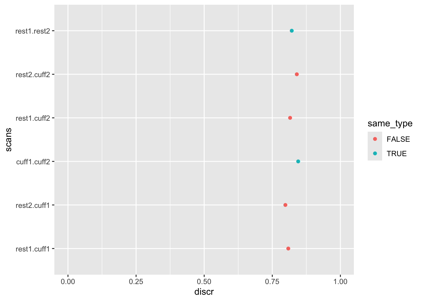

Overall, discriminability is around 0.8, with at most minor differences between different pairings of runs.

17.2 Considerations While Working on the Project

17.2.1 Mislabeled Schaefer Atlas

Two of the pre-computed connectivity matrices are based on Schaefer’s atlas. Unfortunately, the labels are stored incorrectly, as described in this issue. The fix is relatively straightforward. Here, we download the file referenced in that issue, which contains a mapping between the current and correct labels.

label_mapping <- arrow::read_tsv_arrow(
  "https://github.com/user-attachments/files/22352624/labels_mapping.tsv",
  schema = schema(current = int64(), correct = int64()), # specifying to make the join below easier
  skip = 1,
  as_data_frame = FALSE
)
head(label_mapping)

Table
6 rows x 2 columns
$current <int64>
$correct <int64>

We can use those labels to remap the existing source and target columns, as in the code chunk below. Note that the chunk below does this for the schaefer_nrois-400_resolution-2_networks-7 atlas, but it will also need to be done for the schaefer_nrois-400_resolution-2_networks-17 atlas.

open_dataset(
  "data/pre-surgery/mris/derivatives/fcn/connectivity"
) |>
  filter(atlas == "schaefer_nrois-400_resolution-2_networks-7") |>
  left_join(label_mapping, by = join_by(source == current)) |>
  left_join(
    label_mapping,
    by = join_by(target == current),
    suffix = c(".source", ".target")
  ) |>
  select(-source, -target) |>
  rename(source = correct.source, target = correct.target) |>
  head() |>
  collect()

connectivity	sub	ses	task	run	atlas	estimator	source	target
0.6768990	10003	V1	cuff	1	schaefer_nrois-400_resolution-2_networks-7	ledoit_wolf	1	2
0.6125918	10003	V1	cuff	1	schaefer_nrois-400_resolution-2_networks-7	ledoit_wolf	1	3
0.6882472	10003	V1	cuff	1	schaefer_nrois-400_resolution-2_networks-7	ledoit_wolf	1	4
0.5958827	10003	V1	cuff	1	schaefer_nrois-400_resolution-2_networks-7	ledoit_wolf	1	5
0.4730263	10003	V1	cuff	1	schaefer_nrois-400_resolution-2_networks-7	ledoit_wolf	1	6
0.1177192	10003	V1	cuff	1	schaefer_nrois-400_resolution-2_networks-7	ledoit_wolf	1	7

17.2.2 Variability Across Scanners

Many MRI biomarkers exhibit variability across the scanners, which may confound some analyses. For an up-to-date assessment of the issue and overview of current thinking, please see Appendix D.

17.2.3 Data Quality

As with any MRI derivative, all pipeline derivatives have been included. This means that products were included regardless of their quality, and so some products may have been generated from images that are known to have poor quality—rated “red”, or incomparable. For details on the ratings and how to exclude them, see Appendix A. Additionally, extensive QC has not yet been performed on the derivatives themselves, and so there may be cases where pipelines produced atypical outputs. For an overview of planned checks, see Confluence.

17.2.4 Citations

In publications or presentations including data from A2CPS, please include the following statement as attribution:

Data were provided (in part) by the A2CPS Consortium funded by the National Institutes of Health (NIH) Common Fund, which is managed by the Office of the Director (OD)/Office of Strategic Coordination (OSC). Consortium components and their associated funding sources include Clinical Coordinating Center (U24NS112873), Data Integration and Resource Center (U54DA049110), Omics Data Generation Centers (U54DA049116, U54DA049115, U54DA049113), Multi-site Clinical Center 1 (MCC1) (UM1NS112874), and Multi-site Clinical Center 2 (MCC2) (UM1NS118922).

Note

The following published papers should be cited when referring to A2CPS Protocol and Biomarkers: Sluka et al. (2023) Berardi et al. (2022)

Berardi, G., Frey-Law, L., Sluka, K. A., Bayman, E. O., Coffey, C. S., Ecklund, D., Vance, C. G. T., Dailey, D. L., Burns, J., Buvanendran, A., McCarthy, R. J., Jacobs, J., Zhou, X. J., Wixson, R., Balach, T., Brummett, C. M., Clauw, D., Colquhoun, D., Harte, S. E., … Wandner, L. D. (2022). Multi-site observational study to assess biomarkers for susceptibility or resilience to chronic pain: The acute to chronic pain signatures (A2CPS) study protocol. Frontiers in Medicine, 9. https://doi.org/10.3389/fmed.2022.849214

Sluka, K. A., Wager, T. D., Sutherland, S. P., Labosky, P. A., Balach, T., Bayman, E. O., Berardi, G., Brummett, C. M., Burns, J., Buvanendran, A., et al. (2023). Predicting chronic postsurgical pain: Current evidence and a novel program to develop predictive biomarker signatures. Pain, 164(9), 1912–1926. https://doi.org/10.1097/j.pain.0000000000002938

Sadil, P., Arfanakis, K., Bhuiyan, E. H., Caffo, B., Calhoun, V. D., Clauw, D. J., DeLano, M. C., Ford, J. C., Gattu, R., Guo, X., Harris, R. E., Ichesco, E., Johnson, M. A., Jung, H., Kahn, A. B., Kaplan, C. M., Leloudas, N., Lindquist, M. A., Luo, Q., … Chronic Pain Signatures Consortium, T. A. to. (2024). Image processing in the acute to chronic pain signatures (A2CPS) project. bioRxiv. https://doi.org/10.1101/2024.12.19.627509

When using neuroimaging derivatives, please also cite Sadil et al. (2024).