[[12]{.chapter-number}  [EDDY QC]{.chapter-title}]{#sec-eddyqc .quarto-section-identifier}

12 EDDY QC

library(dplyr)
library(fs)
library(ggdist)
library(ggplot2)
library(jsonlite)
library(purrr)
library(tidyr)

This kit reviews the key quality control metrics provided by FSL’s EDDY QC (Bastiani et al., 2019), which are included in A2CPS data releases.

Diffusion MRI (dMRI) is highly sensitive to macroscopic head motion and to eddy currents—rapidly changing magnetic gradients that cause geometric distortions and blurring in the reconstructed images. FSL’s EDDY tool is a gold-standard approach for correcting these artifacts. As a byproduct of the correction process, EDDY generates several quantitative quality control metrics. While these metrics are not used in the automated rating of dMRI images in A2CPS, they provide valuable, objective information about the severity of movement and magnetic susceptibility artifacts on a scan (e.g., Contrast-to-Noise Ratio).

12.1 Starting Project

12.1.1 Locate Data

On TACC, the data are stored underneath the releases. For example, data release v2.1.0 is underneath

/corral-secure/projects/A2CPS/products/consortium-data/pre-surgery-release-2-1-0

Paths in this kit are written relative to that release folder, so the neuroimaging data are underneath mris.

The outputs are organized by participant and session¹.

¹ Note that the directory structure varies across participants, with some participants matching sub-[recordid]/ses-[visit]/[contents] and others matching sub-[recordid]/ses-[visit]/eddyqc/[contents].

$ ls mris/derivatives/eddyqc/ | head
sub-10003
sub-10008
sub-10010
sub-10011
sub-10013
sub-10014
sub-10015
sub-10017
sub-10020
sub-10023

$ tree mris/derivatives/eddyqc/sub-10003
sub-10003
└── ses-V1
    ├── avg_b0_pe0.png
    ├── avg_b0.png
    ├── avg_b1000.png
    ├── avg_b2000.png
    ├── avg_b3000.png
    ├── avg_b500.png
    ├── cnr0000.nii.gz.png
    ├── cnr0001.nii.gz.png
    ├── cnr0002.nii.gz.png
    ├── cnr0003.nii.gz.png
    ├── cnr0004.nii.gz.png
    ├── qc.json
    ├── qc.pdf
    ├── ref_list.png
    ├── ref.txt
    └── vdm.png

1 directory, 16 files

The pdf is a visual report summarizing the scan quality, including tables with quantitative metrics and images indicating scan quality. The metrics are available in the json, along with metadata about the scan.

12.1.2 Extract Data

Let’s collate the QC metrics into a single table. To do so, we recursively search for and read the qc.json files.

qcs <- tibble(
  src = dir_ls(
    "data/pre-surgery/mris/derivatives/eddyqc",
    recurse = TRUE,
    glob = "*qc.json"
  )
) |>
  mutate(
    qc = map(
      src,
      \(x) read_json(x, simplifyVector = TRUE),
      .progress = TRUE
    )
  )
# let's look at the fields on one of those qc.json files
qcs$qc[[1]] |> names()

 [1] "data_eddy_para"        "data_file_bvals"       "data_file_eddy"       
 [4] "data_file_mask"        "data_no_PE_dirs"       "data_no_b0_vols"      
 [7] "data_no_dw_vols"       "data_no_shells"        "data_protocol"        
[10] "data_unique_bvals"     "data_unique_pes"       "data_vox_size"        
[13] "eddy_input"            "eddy_input_flag"       "qc_cnr_avg"           
[16] "qc_cnr_flag"           "qc_cnr_std"            "qc_field_flag"        
[19] "qc_mot_abs"            "qc_mot_rel"            "qc_ol_flag"           
[22] "qc_outliers_b"         "qc_outliers_pe"        "qc_outliers_tot"      
[25] "qc_params_avg"         "qc_params_flag"        "qc_path"              
[28] "qc_rss_flag"           "qc_s2v_params_avg_std" "qc_s2v_params_flag"   
[31] "qc_vox_displ_std"

In these qc.json files, there are three kinds of fields: data_* fields, which describe the scan, eddy_* fields, which describe how EDDY was configured, and qc_* fields, which summarize the scan quality. Let’s dig into qc_cnr_avg. That field is a vector with a length equal to the number of shells in the scan. The entries are the average angular Contrast-to-Noise ratio, which is a standardized measure of scan quality (Bastiani et al., 2019)²

² The first entry corresponds to the b0, and so it is really as signal-to-noise ratio rather than a traditional angular CNR.

cnr <- qcs |>
  mutate(
    qc = map(
      qc,
      \(x) tibble(CNR = x$qc_cnr_avg, b = c(0, 500, 1000, 2000, 3000))
    )
  ) |>
  unnest(qc) |>
  filter(CNR > 0) # 0 indicates some failure in calculation of the metric
head(cnr)

src	CNR	b
data/pre-surgery/mris/derivatives/eddyqc/sub-10008/ses-V1/qc.json	11.36	0
data/pre-surgery/mris/derivatives/eddyqc/sub-10008/ses-V1/qc.json	0.74	500
data/pre-surgery/mris/derivatives/eddyqc/sub-10008/ses-V1/qc.json	0.98	1000
data/pre-surgery/mris/derivatives/eddyqc/sub-10008/ses-V1/qc.json	2.28	2000
data/pre-surgery/mris/derivatives/eddyqc/sub-10008/ses-V1/qc.json	3.26	3000
data/pre-surgery/mris/derivatives/eddyqc/sub-10010/ses-V1/qc.json	3.89	0

Now, plot the ratios by b-value.

cnr |>
  mutate(b = factor(b)) |> # to make plotting nicer
  ggplot(aes(y = b, x = CNR)) +
  stat_dotsinterval(quantiles = 100) +
  scale_x_log10("CNR/SNR")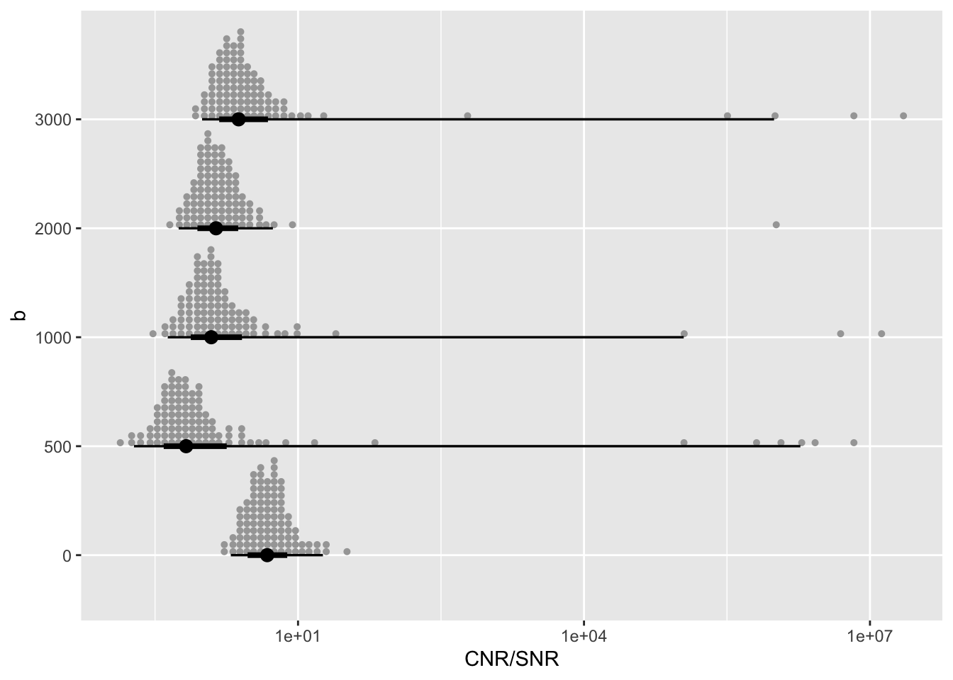

Generally, the angular CNR seems to increase with increasing b-value. There are also some outliers, which likely correspond to preprocessing failures.

12.2 Considerations While Working on the Project

12.2.1 Effective vs. Raw CNR

To enable comparisons of quality across datasets, it is recommended to convert the CNR values output by EDDY into “effective CNR” values by the square root of the number of acquired volumes and dividing it by the voxel volume (Bastiani et al., 2019).

12.2.2 Background

For detailed information about all the QC metrics provided, please see official FSL documentation for EDDY QC, along with the report Bastiani et al. (2019).

12.2.3 Citations

If you use these derivatives please cite the EDDY QC paper (Bastiani et al., 2019).

Bastiani, M., Cottaar, M., Fitzgibbon, S. P., Suri, S., Alfaro-Almagro, F., Sotiropoulos, S. N., Jbabdi, S., & Andersson, J. L. (2019). Automated quality control for within and between studies diffusion MRI data using a non-parametric framework for movement and distortion correction. Neuroimage, 184, 801–812. https://doi.org/10.1016/j.neuroimage.2018.09.073

In publications or presentations including data from A2CPS, please include the following statement as attribution:

Data were provided (in part) by the A2CPS Consortium funded by the National Institutes of Health (NIH) Common Fund, which is managed by the Office of the Director (OD)/Office of Strategic Coordination (OSC). Consortium components and their associated funding sources include Clinical Coordinating Center (U24NS112873), Data Integration and Resource Center (U54DA049110), Omics Data Generation Centers (U54DA049116, U54DA049115, U54DA049113), Multi-site Clinical Center 1 (MCC1) (UM1NS112874), and Multi-site Clinical Center 2 (MCC2) (UM1NS118922).

Note

The following published papers should be cited when referring to A2CPS Protocol and Biomarkers: Sluka et al. (2023) Berardi et al. (2022)

Berardi, G., Frey-Law, L., Sluka, K. A., Bayman, E. O., Coffey, C. S., Ecklund, D., Vance, C. G. T., Dailey, D. L., Burns, J., Buvanendran, A., McCarthy, R. J., Jacobs, J., Zhou, X. J., Wixson, R., Balach, T., Brummett, C. M., Clauw, D., Colquhoun, D., Harte, S. E., … Wandner, L. D. (2022). Multi-site observational study to assess biomarkers for susceptibility or resilience to chronic pain: The acute to chronic pain signatures (A2CPS) study protocol. Frontiers in Medicine, 9. https://doi.org/10.3389/fmed.2022.849214

Sluka, K. A., Wager, T. D., Sutherland, S. P., Labosky, P. A., Balach, T., Bayman, E. O., Berardi, G., Brummett, C. M., Burns, J., Buvanendran, A., et al. (2023). Predicting chronic postsurgical pain: Current evidence and a novel program to develop predictive biomarker signatures. Pain, 164(9), 1912–1926. https://doi.org/10.1097/j.pain.0000000000002938

Sadil, P., Arfanakis, K., Bhuiyan, E. H., Caffo, B., Calhoun, V. D., Clauw, D. J., DeLano, M. C., Ford, J. C., Gattu, R., Guo, X., Harris, R. E., Ichesco, E., Johnson, M. A., Jung, H., Kahn, A. B., Kaplan, C. M., Leloudas, N., Lindquist, M. A., Luo, Q., … Chronic Pain Signatures Consortium, T. A. to. (2024). Image processing in the acute to chronic pain signatures (A2CPS) project. bioRxiv. https://doi.org/10.1101/2024.12.19.627509

When using neuroimaging derivatives, please also cite Sadil et al. (2024).