library(readr)
library(ggplot2)
library(dplyr)
library(tidyr)6 Brain Age
This starter kit walk through the “Brain Age” outputs that have been derived from the anatomical scans. The examples in the kit rely on bash and R.
Fundamentally brainager calculations are about producing an estimated age based on measurable characteristics of a brain image, such as regional variations in gray matter density. The difference between estimated and chronological age is often referred to in the literature as the “brain age gap” (BAG) or “predicted age difference” (PAD), and is usually expressed as estimated minus chronological age. This value is often interpreted as an indicator of brain health.
6.1 Starting Project
6.1.1 Locate data
In the release folder, data are stored underneath the mris/derivatives folder:
/corral-secure/projects/A2CPS/products/consortium-data/pre-surgery/mris/derivatives/brainager6.1.2 Extract data
Data for each participant are stored in a sub-directory.
$ ls | head
sub-10003
sub-10005
sub-10008
sub-10010
sub-10011
sub-10013
sub-10014
sub-10015
sub-10017
sub-10020
For example1:
1 The tree command is just used here to display the folder structure, and is not required for you to have.
$ tree sub-10319
sub-10319
└── ses-V1
├── slicesdir_sub-10319_ses-V1_T1w.nii
│   ├── index.html
│   ├── _tmp_tmph17ksnl8_c1sub-10319_ses-V1_T1w.png
│   ├── _tmp_tmph17ksnl8_c2sub-10319_ses-V1_T1w.png
│   ├── _tmp_tmph17ksnl8_c3sub-10319_ses-V1_T1w.png
│   ├── _tmp_tmph17ksnl8_smwc1sub-10319_ses-V1_T1w.png
│   ├── _tmp_tmph17ksnl8_smwc2sub-10319_ses-V1_T1w.png
│   └── _tmp_tmph17ksnl8_smwc3sub-10319_ses-V1_T1w.png
├── sub-10319_ses-V1_T1w.m
├── sub-10319_ses-V1_T1w_tissue_volumes.tsv
└── sub-10319_ses-V1_T1w.tsv

2 directories, 10 files
Most users will be interested in the predicted ages, which can be found in sub-[recordid]/ses-[protocolid]/sub-[recordid]_ses-[protocolid]_T1w.tsv. For example
$ cat sub-10003/ses-V1/sub-10003_ses-V1_T1w.tsv
File    brain.predicted_age lower.CI    upper.CI
sub-10003_ses-V1_T1w    73.6037 72.9683 74.2392
Here is an example of how these files could be loaded using R.
# list all files
files <- fs::dir_ls("data/brainager", glob = "*T1w.tsv", recurse = TRUE)

# read in all tsvs
ages <- readr::read_tsv(files)
ages
# A tibble: 1,017 × 4
File brain.predicted_age lower.CI upper.CI
<chr> <dbl> <dbl> <dbl>
1 sub-10003_ses-V1_T1w 73.6 73.0 74.2
2 sub-10005_ses-V1_T1w 65.7 64.6 66.9
3 sub-10008_ses-V1_T1w 75.5 74.7 76.3
4 sub-10010_ses-V1_T1w 44.6 42.6 46.5
5 sub-10011_ses-V1_T1w 40.5 38.5 42.4
6 sub-10013_ses-V1_T1w 72.1 71.5 72.8
7 sub-10014_ses-V1_T1w 42.3 41.7 42.9
8 sub-10015_ses-V1_T1w 55.0 53.2 56.8
9 sub-10017_ses-V1_T1w 57.9 57.2 58.7
10 sub-10020_ses-V1_T1w 59.2 58.6 59.7
# ℹ 1,007 more rowsThe column File identifies the anatomical image that was used for to make the prediction. When working with other A2CPS data, it may be helpful to extract the subject ID.
ages_with_sub <- ages |>
  dplyr::mutate(
    sub = stringr::str_extract(File, "[[:digit:]]{5}") |> as.integer(),
  )
ages_with_sub
# A tibble: 1,017 × 5
File brain.predicted_age lower.CI upper.CI sub
<chr> <dbl> <dbl> <dbl> <int>
1 sub-10003_ses-V1_T1w 73.6 73.0 74.2 10003
2 sub-10005_ses-V1_T1w 65.7 64.6 66.9 10005
3 sub-10008_ses-V1_T1w 75.5 74.7 76.3 10008
4 sub-10010_ses-V1_T1w 44.6 42.6 46.5 10010
5 sub-10011_ses-V1_T1w 40.5 38.5 42.4 10011
6 sub-10013_ses-V1_T1w 72.1 71.5 72.8 10013
7 sub-10014_ses-V1_T1w 42.3 41.7 42.9 10014
8 sub-10015_ses-V1_T1w 55.0 53.2 56.8 10015
9 sub-10017_ses-V1_T1w 57.9 57.2 58.7 10017
10 sub-10020_ses-V1_T1w 59.2 58.6 59.7 10020
# ℹ 1,007 more rows6.2 Considerations While Working on the Project
It is in principle possible to replicate the processing that was used in a release by running the brainageR container2 on the raw data. However, A2CPS Releases 1.0.0, 1.1.0, and 2.0.0 have not included raw T1w files for privacy reasons, and thus the end result may differ from the released version, which was generated on the raw images.
2 The container used by A2CPS is available here.
6.2.1 Variability Across Scanners
Many MRI biomarkers exhibit variability across the scanners, which may confound some analyses. For an up-to-date assessment of the issue and overview of current thinking, please see Confluence.
6.2.2 Data Quality
As with any MRI derivative, all pipeline derivatives have been included. This means that products were included regardless of their quality, and so some products may have been generated from images that are known to have poor quality—rated “red”, or incomparable. For details on the ratings and how to exclude them, see Appendix A. Additionally, extensive QC has not yet been performed on the derivatives themselves, and so there may be cases where pipelines produced atypical outputs. For an overview of planned checks, see Confluence.
6.2.3 Calculating the Brain Age Gap
Predicted ages are neat, but these values are most useful when compared against a participant’s chronological age. These can be found in the demographics portion of the release.
baseline_ages <- read_csv(
  "data/demographics/demographics-2025-01-10.csv",
  col_select = c("record_id", "age")
)

brainage <- ages_with_sub |>
  left_join(baseline_ages, by = join_by(sub == record_id)) |>
  mutate(
    brain_age_gap = brain.predicted_age - age
  ) |>
  filter(!is.na(age)) # age not available for all participants
brainage
# A tibble: 996 × 7
File brain.predicted_age lower.CI upper.CI sub age brain_age_gap
<chr> <dbl> <dbl> <dbl> <dbl> <dbl> <dbl>
1 sub-10003_se… 73.6 73.0 74.2 10003 73 0.604
2 sub-10005_se… 65.7 64.6 66.9 10005 58 7.73
3 sub-10008_se… 75.5 74.7 76.3 10008 73 2.49
4 sub-10010_se… 44.6 42.6 46.5 10010 64 -19.4
5 sub-10011_se… 40.5 38.5 42.4 10011 54 -13.5
6 sub-10013_se… 72.1 71.5 72.8 10013 71 1.14
7 sub-10014_se… 42.3 41.7 42.9 10014 45 -2.70
8 sub-10015_se… 55.0 53.2 56.8 10015 65 -9.98
9 sub-10017_se… 57.9 57.2 58.7 10017 56 1.95
10 sub-10020_se… 59.2 58.6 59.7 10020 53 6.17
# ℹ 986 more rowsBy plotting the predicted ages against the true ages, we can review the accuracy of the predictions.
lm_eqn <- function(fit) {
  eq <- substitute(
    italic(y) == a + b %.% italic(age) * "," ~ ~ italic(r)^2 ~ "=" ~ r2,
    list(
      a = format(unname(coef(fit)[1]), digits = 2),
      b = format(unname(coef(fit)[2]), digits = 2),
      r2 = format(summary(fit)$r.squared, digits = 3)
    )
  )
  as.character(as.expression(eq))
}

fit <- lm(brain.predicted_age ~ age, data = brainage)

brainage |>
  ggplot(aes(x = age, y = brain.predicted_age)) +
  geom_abline() +
  geom_point(alpha = 0.5) +
  geom_smooth(method = "lm", formula = y ~ x) +
  coord_fixed() +
  geom_text(x = 40, y = 80, label = lm_eqn(fit), parse = TRUE)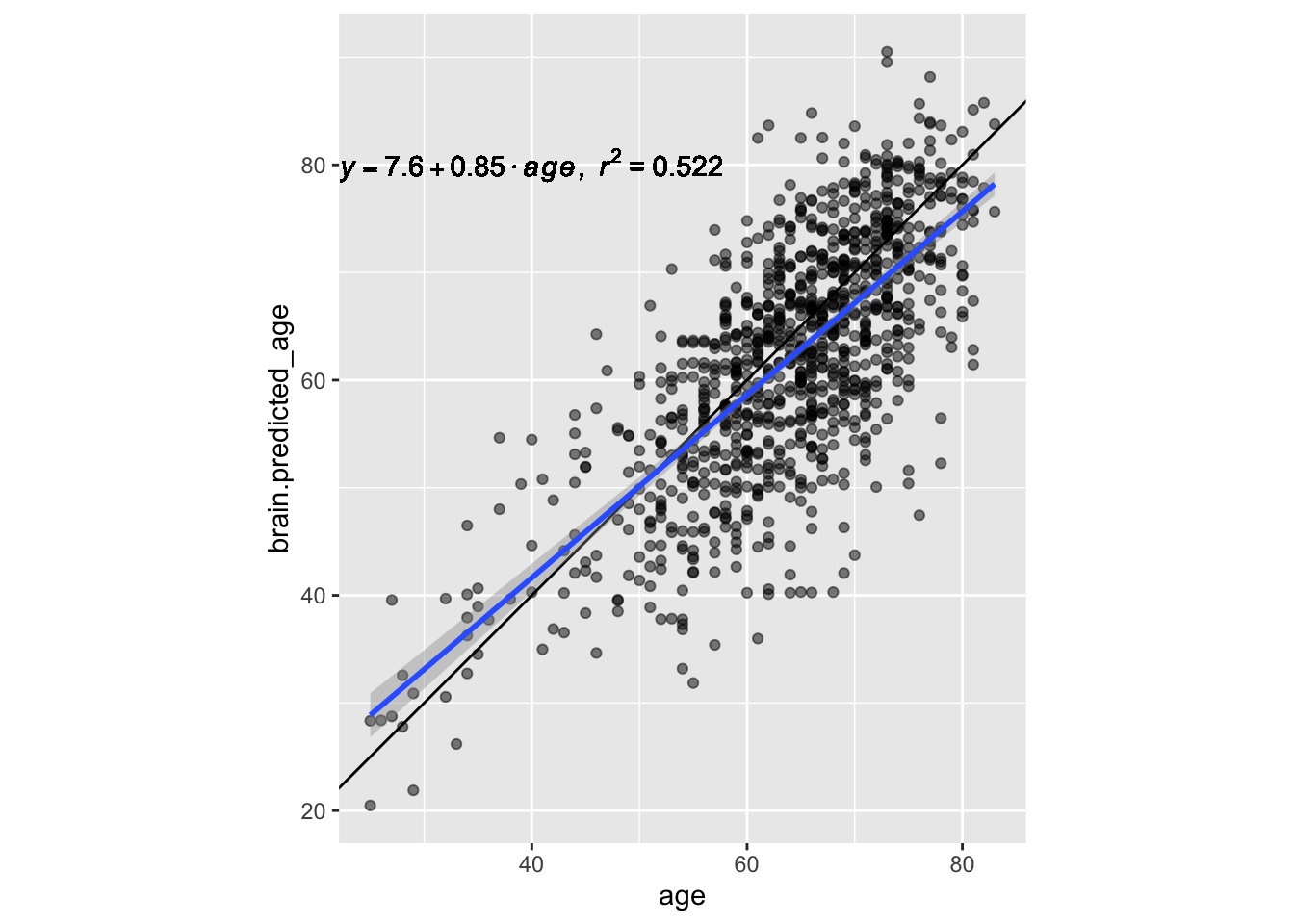
The “brain age gap” is the difference between predicted and true age. Positive gaps indicate “older” brains, and younger gaps indicate “younger” brains.
brainage |>
  ggplot(aes(x = brain_age_gap)) +
  geom_histogram() +
  xlab("(<-- Younger) Brain Age Gap (Older -->)")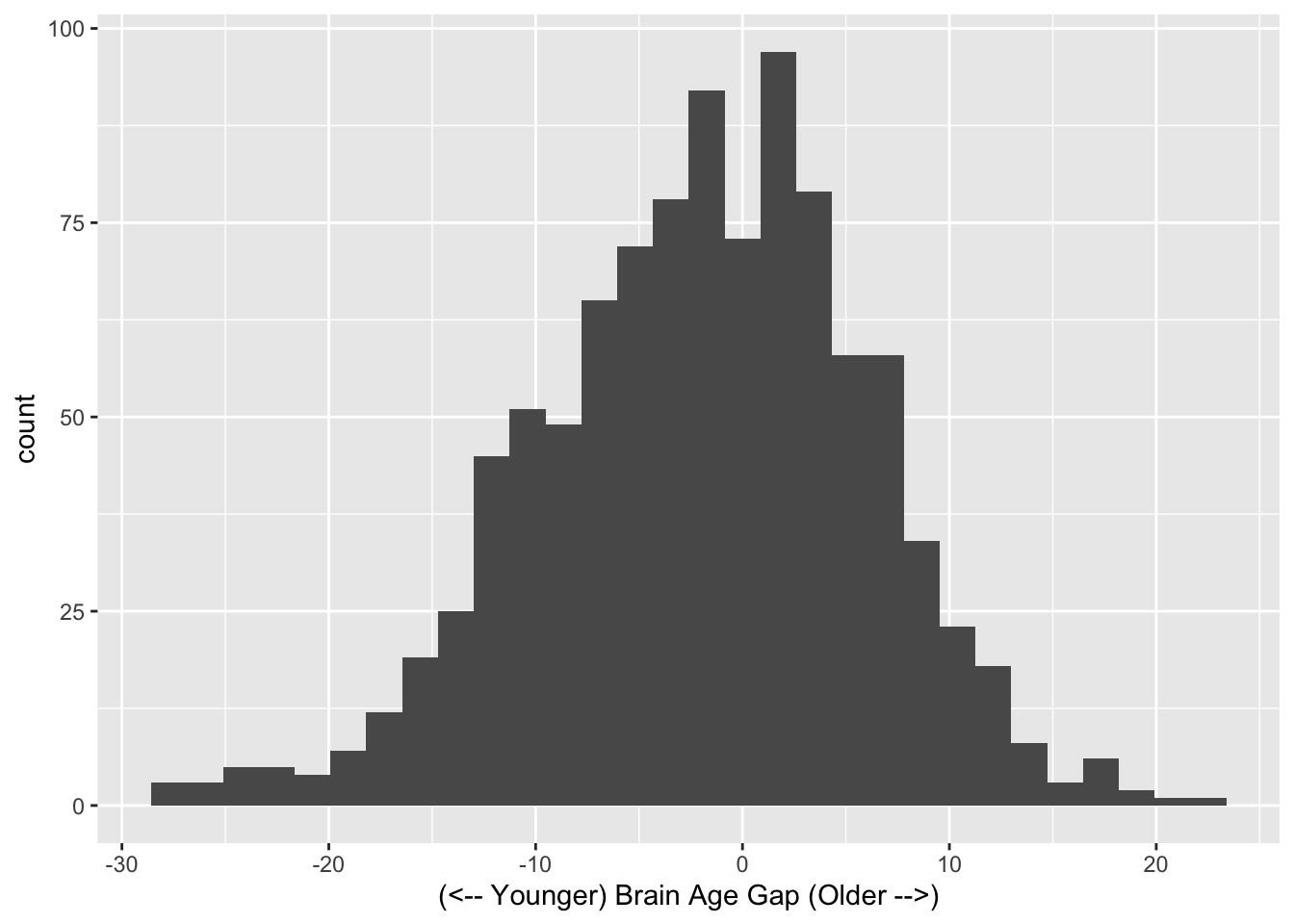
6.2.4 Correction
Note that using the raw Brain Age Gap can be problematic, and, for final analyses, it is typical to calculate a derivative that has been “corrected”. The issue is that the predictions tend to be worse for the youngest and oldest people – and so the gap is related to age (e.g., a relationship with larger raw gaps partly reflects a relationship with true age).
brainage |>
  ggplot(aes(x = age, y = brain_age_gap)) +
  geom_point(alpha = 0.5) +
  geom_smooth(method = "lm", formula = y ~ x) +
  coord_fixed()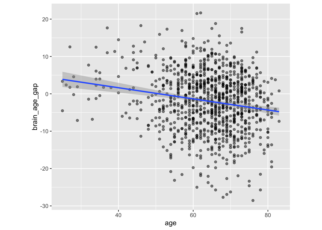
Corrections aim to make them independent, by, for example, residualizing. See Smith et al. (2019).
Smith, S. M., Vidaurre, D., Alfaro-Almagro, F., Nichols, T. E., & Miller, K. L. (2019). Estimation of brain age delta from brain imaging. Neuroimage, 200, 528–539. https://doi.org/10.1016/j.neuroimage.2019.06.017
bag_age_fit <- lm(brain_age_gap ~ age, data = brainage)

brainage |>
  mutate(
    brain_age_gap_corrected = residuals(bag_age_fit),
    brain_age_gap = scale(brain_age_gap, scale = FALSE)
  ) |>
  select(sub, brain_age_gap, brain_age_gap_corrected) |>
  ggplot(aes(x = brain_age_gap, y = brain_age_gap_corrected)) +
  geom_point(alpha = 0.5) +
  geom_abline() +
  geom_smooth(method = "lm", formula = y ~ x)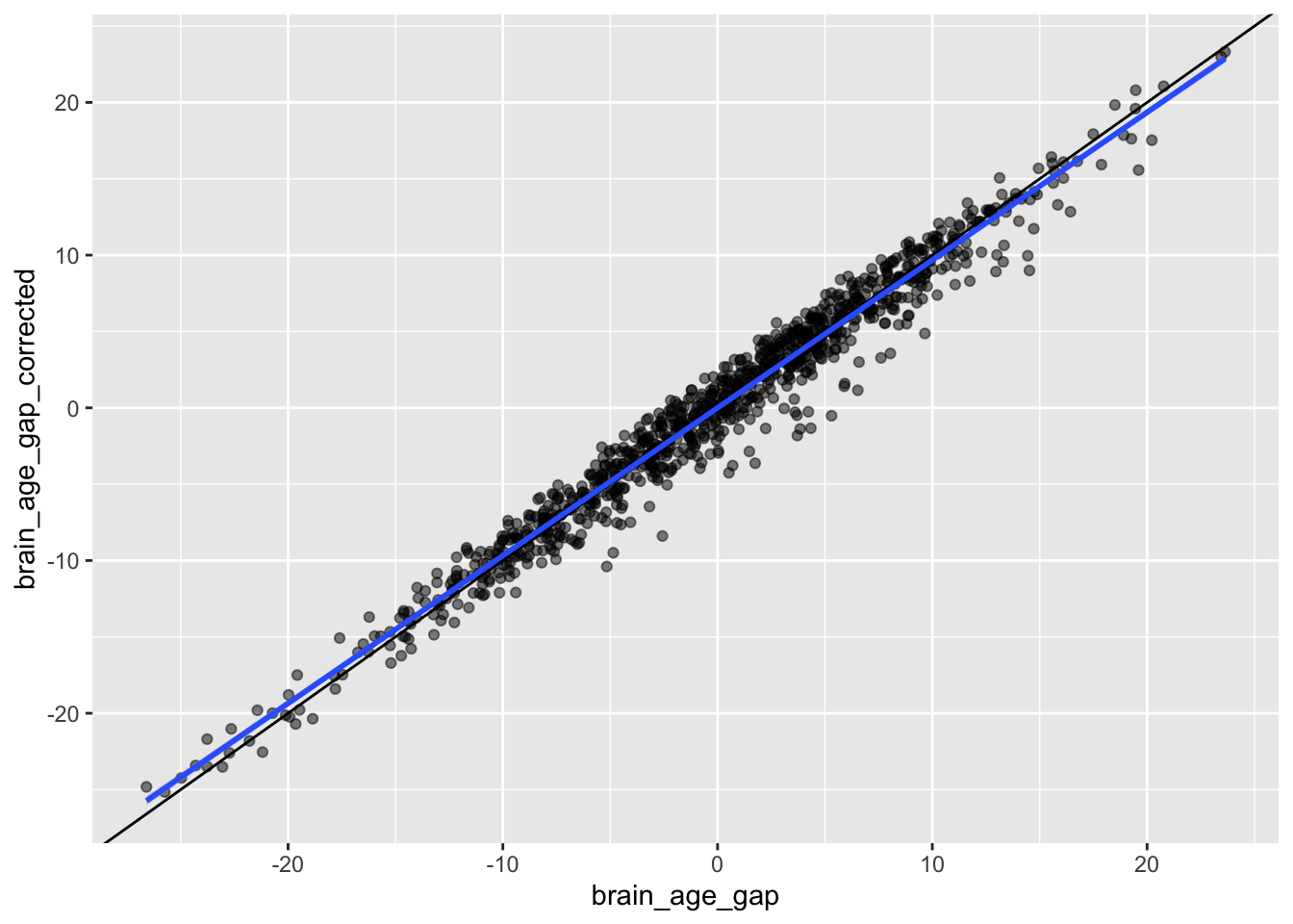
6.2.5 Other Models
There are many models for calculating Brain Age. The values that have been pre-calculated for A2CPS are derived from a model that has been around for a while and used successfully in a variety of studies (Biondo et al., 2022; Clausen et al., 2022; Hobday et al., 2022). For some analyses, it may be worthwhile to assess whether results persist across different models. For pain studies, one successful model has been DeepBrainNet (Bashyam et al., 2020; Montesino-Goicolea et al., 2023; Valdes-Hernandez et al., 2023), which can be used with derivatives from fMRIPrep.
Biondo, F., Jewell, A., Pritchard, M., Aarsland, D., Steves, C. J., Mueller, C., & Cole, J. H. (2022). Brain-age is associated with progression to dementia in memory clinic patients. NeuroImage: Clinical, 36, 103175. https://doi.org/10.1016/j.nicl.2022.103175
Clausen, A. N., Fercho, K. A., Monsour, M., Disner, S., Salminen, L., Haswell, C. C., Rubright, E. C., Watts, A. A., Buckley, M. N., Maron-Katz, A., et al. (2022). Assessment of brain age in posttraumatic stress disorder: Findings from the ENIGMA PTSD and brain age working groups. Brain and Behavior, 12(1), e2413. https://doi.org/10.1002/brb3.2413
Hobday, H., Cole, J. H., Stanyard, R. A., Daws, R. E., Giampietro, V., O’Daly, O., Leech, R., & Váša, F. (2022). Tissue volume estimation and age prediction using rapid structural brain scans. Scientific Reports, 12(1), 12005.
Bashyam, V. M., Erus, G., Doshi, J., Habes, M., Nasrallah, I. M., Truelove-Hill, M., Srinivasan, D., Mamourian, L., Pomponio, R., Fan, Y., et al. (2020). MRI signatures of brain age and disease over the lifespan based on a deep brain network and 14 468 individuals worldwide. Brain, 143(7), 2312–2324. https://doi.org/10.1093/brain/awaa160
Montesino-Goicolea, S., Valdes-Hernandez, P., Nodarse, C. L., Johnson, A. J., Cole, J. H., Antoine, L. H., Goodin, B. R., Fillingim, R. B., & Cruz-Almeida, Y. (2023). Brain-predicted age difference mediates the association between PROMIS sleep impairment, and self-reported pain measure in persons with knee pain. Aging Brain, 4, 100088. https://doi.org/10.1016/j.nbas.2023.100088
Valdes-Hernandez, P. A., Nodarse, C. L., Johnson, A. J., Montesino-Goicolea, S., Bashyam, V., Davatzikos, C., Peraza, J. A., Cole, J. H., Huo, Z., Fillingim, R. B., et al. (2023). Brain-predicted age difference estimated using DeepBrainNet is significantly associated with pain and function—a multi-institutional and multiscanner study. Pain, 164(12), 2822–2838. https://doi.org/10.1097/j.pain.0000000000002984
6.2.6 Methods
For additional documentation on the files and a detailed description of the methods, please see the official brainageR repo.
6.2.7 Citations
If you use the brainageR materials, please follow the instructions for citing the brainageR package: https://github.com/james-cole/brainageR?tab=readme-ov-file#citations.
In publications or presentations including data from A2CPS, please include the following statement as attribution:
Data were provided [in part] by the A2CPS Consortium funded by the National Institutes of Health (NIH) Common Fund, which is managed by the Office of the Director (OD)/ Office of Strategic Coordination (OSC). Consortium components and their associated funding sources include Clinical Coordinating Center (U24NS112873), Data Integration and Resource Center (U54DA049110), Omics Data Generation Centers (U54DA049116, U54DA049115, U54DA049113), Multi-site Clinical Center 1 (MCC1) (UM1NS112874), and Multi-site Clinical Center 2 (MCC2) (UM1NS118922).
Note
Berardi, G., Frey-Law, L., Sluka, K. A., Bayman, E. O., Coffey, C. S., Ecklund, D., Vance, C. G. T., Dailey, D. L., Burns, J., Buvanendran, A., McCarthy, R. J., Jacobs, J., Zhou, X. J., Wixson, R., Balach, T., Brummett, C. M., Clauw, D., Colquhoun, D., Harte, S. E., … Wandner, L. D. (2022). Multi-site observational study to assess biomarkers for susceptibility or resilience to chronic pain: The acute to chronic pain signatures (A2CPS) study protocol. Frontiers in Medicine, 9. https://doi.org/10.3389/fmed.2022.849214
Sluka, K. A., Wager, T. D., Sutherland, S. P., Labosky, P. A., Balach, T., Bayman, E. O., Berardi, G., Brummett, C. M., Burns, J., Buvanendran, A., et al. (2023). Predicting chronic postsurgical pain: Current evidence and a novel program to develop predictive biomarker signatures. Pain, 164(9), 1912–1926. https://doi.org/10.1097/j.pain.0000000000002938
Sadil, P., Arfanakis, K., Bhuiyan, E. H., Caffo, B., Calhoun, V. D., Clauw, D. J., DeLano, M. C., Ford, J. C., Gattu, R., Guo, X., Harris, R. E., Ichesco, E., Johnson, M. A., Jung, H., Kahn, A. B., Kaplan, C. M., Leloudas, N., Lindquist, M. A., Luo, Q., … Chronic Pain Signatures Consortium, T. A. to. (2024). Image processing in the acute to chronic pain signatures (A2CPS) project. bioRxiv. https://doi.org/10.1101/2024.12.19.627509
When using imaging derivatives, please also cite Sadil et al. (2024).