[[10]{.chapter-number}  [ICA Connectivity]{.chapter-title}]{#sec-postgift .quarto-section-identifier}

10 ICA Connectivity

library(readr)
library(dplyr)
library(ggplot2)
library(duckplyr)
library(fs)
library(tidyr)
library(ggdist)

The Chapter 9 products provide outputs in a raw format that will be familiar to users of that library. To facilitate analyses, A2CPS has repackaged those products into a tabular format. This kit covers the repackaged structure.

10.1 Starting Project

10.1.1 Locate Data

On TACC, the neuroimaging data are stored underneath the releases. For example, data release v2.#.# is underneath

pre-surgery/mris

The MRIQC metrics are underneath derivatives/postgift. Let’s take a look.

$ ls postgift
amplitude  amplitude.json  biomarkers  biomarkers.json  connectivity  connectivity.json

10.1.2 Extract Data

The tabular data comprise parquet files that have been partitioned in a hive style. Each table is a different summary of the components derived from GIFT.

amplitude: a measure of component amplitudes. In particular, they are the fractional Amplitude of Low Frequency Fluctuations (Zou et al., 2008).
connectivity: the (product-moment) correlations between component timecourses.
biomarkers: putative biomarkers of chronic pain calculated for A2CPS analyses.

Zou, Q.-H., Zhu, C.-Z., Yang, Y., Zuo, X.-N., Long, X.-Y., Cao, Q.-J., Wang, Y.-F., & Zang, Y.-F. (2008). An improved approach to detection of amplitude of low-frequency fluctuation (ALFF) for resting-state fMRI: Fractional ALFF. Journal of Neuroscience Methods, 172(1), 137–141. https://doi.org/10.1016/j.jneumeth.2008.04.012

Let’s take a look at just the amplitudes.

amplitude <- read_parquet_duckdb(
  dir_ls(
    "data/postgift/amplitude",
    recurse = TRUE,
    glob = "*parquet"
  ),
  prudence = "lavish"
)

head(amplitude)

fALFF	component	sub	ses	task	run	model
2.061823	0	10003	V1	rest	1	2.0
18.220871	1	10003	V1	rest	1	2.0
2.286946	2	10003	V1	rest	1	2.0
9.823509	3	10003	V1	rest	1	2.0
1.624792	4	10003	V1	rest	1	2.0
1.383541	5	10003	V1	rest	1	2.0

To get a feel for the data, let’s see whether there are differences between the amplitudes in the REST1 and CUFF1 scans.

First, we filter the table, keeping only the amplitudes from a single model. We’ll also convert the components into a factor, for later use during modeling. At this point, the dataset is small enough that it’s easy to handle in memory, and so we’ll also collect it.

run1_amplitudes <- amplitude |>
  filter(model == "2.1", run == 1) |>
  select(-model, -run, -ses) |>
  collect() |>
  mutate(component = factor(component))

head(run1_amplitudes)

fALFF	component	sub	task
1.215915	0	10003	cuff
5.390841	1	10003	cuff
2.573948	2	10003	cuff
2.491914	3	10003	cuff
1.392216	4	10003	cuff
1.952687	5	10003	cuff

To get a very high-level overview of the data, generate the MA plot. Let’s exclude the “red” scans to determine whether those are driving the difference.

red_run1_scans <- read_tsv(dir_ls("data/scans", glob = "*tsv"), na = "n/a") |>
  filter(rating == "red", stringr::str_detect(filename, "cuff_run-0[12]")) |>
  mutate(
    sub = stringr::str_extract(filename, "[[:digit:]]{5}") |> as.integer()
  ) |>
  select(sub)

Figure 10.1: Fractional Amplitude of Low Frequency Fluctuations. Each panel is a distinct component. The x-axis is a mean average, and the y-axis is a ratio of the two fALFFs. The

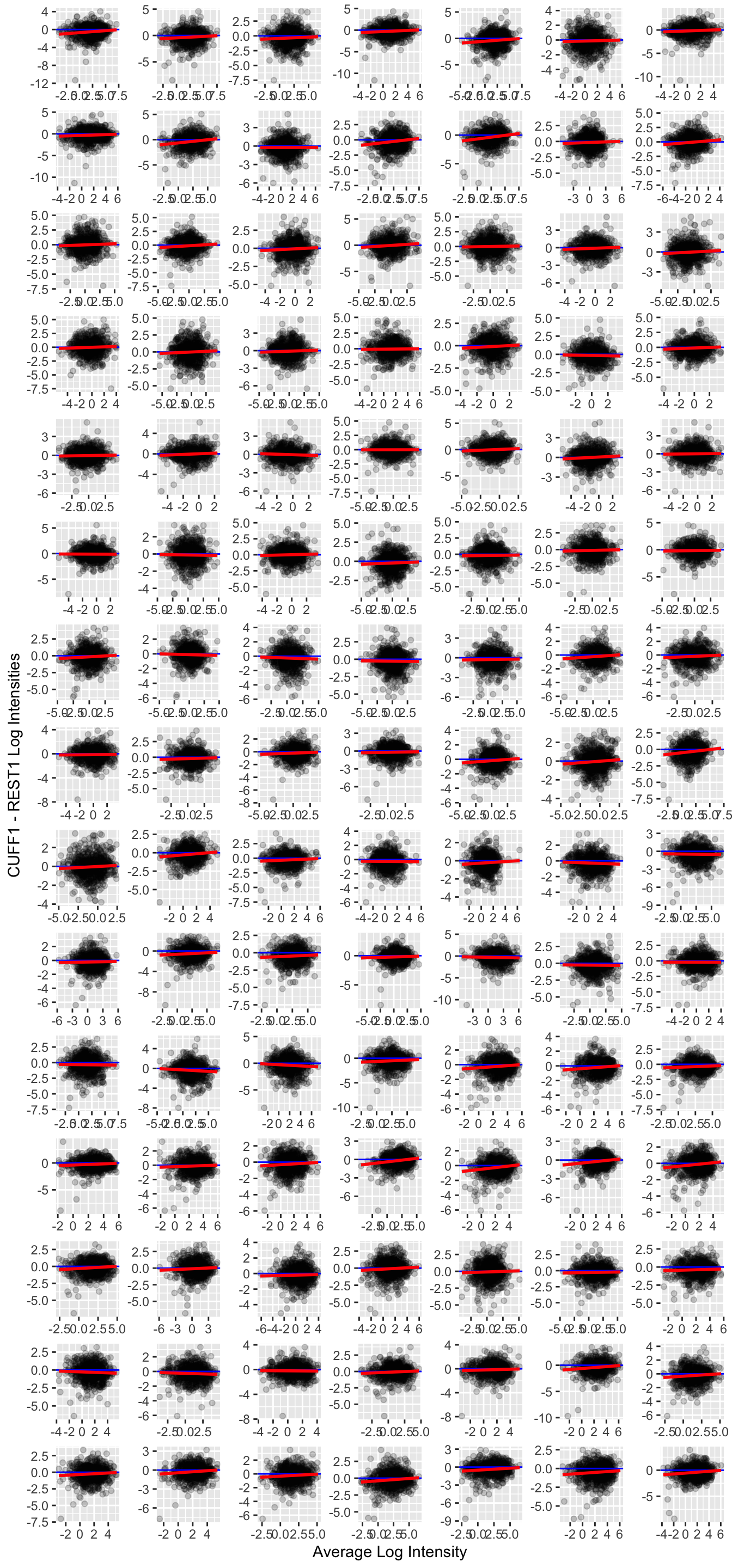
For the most part, there is not a substantially large difference in the log intensities. However, it may be interesting that there appears to be a trend such that amplitudes are somewhat lower in the CUFF as compared to REST conditions.

lme4::lmer(
  log(fALFF) ~ task + (1 | sub) + (1 | component),
  run1_amplitudes_without_red
) |>
  summary()

Linear mixed model fit by REML ['lmerMod']
Formula: log(fALFF) ~ task + (1 | sub) + (1 | component)
   Data: run1_amplitudes_without_red

REML criterion at convergence: 426430.9

Scaled residuals: 
    Min      1Q  Median      3Q     Max 
-5.4681 -0.6343  0.0154  0.6551  5.6997 

Random effects:
 Groups    Name        Variance Std.Dev.
 sub       (Intercept) 0.4852   0.6966  
 component (Intercept) 0.5847   0.7647  
 Residual              0.6963   0.8344  
Number of obs: 170100, groups:  sub, 943; component, 105

Fixed effects:
            Estimate Std. Error t value
(Intercept) 0.560178   0.078077   7.175
taskrest    0.114274   0.004422  25.843

Correlation of Fixed Effects:
         (Intr)
taskrest -0.036

So, indeed, there is some evidence for higher amplitudes during REST1 as compared with CUFF1. Please note that a more careful analysis should include other factors like scanning site, participant age, or motion.

10.2 Considerations While Working on the Project

10.2.1 Variability Across Scanners

Many MRI biomarkers exhibit variability across the scanners, which may confound some analyses. For an up-to-date assessment of the issue and overview of current thinking, please see Confluence.

10.2.2 Data Quality

As with any MRI derivative, all pipeline derivatives have been included. This means that products were included regardless of their quality, and so some products may have been generated from images that are known to have poor quality—rated “red”, or incomparable. For details on the ratings and how to exclude them, see Appendix A. Additionally, extensive QC has not yet been performed on the derivatives themselves, and so there may be cases where pipelines produced atypical outputs. For an overview of planned checks, see Confluence.

10.2.3 Data Generation

These outputs were generated by the postgift_app.

All GIFT outputs rely on the MATLAB toolbox GIFT. The fALFF measures are calculated by icatb_postprocess_timecourses.m. Prior to calculating connectivities, timecourses were despiked and filtered (high-pass Butterworth filter thresholded at 0.15 Hz). Amptlitudes were calculated with frequency limits of 0.1 to 0.15 Hz. Spectra were estimated using a multi-taper (time-bandwidth: 3, K: 5 tapers).

The biomarkers table was calculated by this A2CPS biomarker-extractor workflow. Details of the calculations are provided in the data dictionary.

10.2.4 Citations

If you use these products in your analyses, please cite the relevant papers written by members TReNDS.

In publications or presentations including data from A2CPS, please include the following statement as attribution:

Data were provided [in part] by the A2CPS Consortium funded by the National Institutes of Health (NIH) Common Fund, which is managed by the Office of the Director (OD)/ Office of Strategic Coordination (OSC). Consortium components and their associated funding sources include Clinical Coordinating Center (U24NS112873), Data Integration and Resource Center (U54DA049110), Omics Data Generation Centers (U54DA049116, U54DA049115, U54DA049113), Multi-site Clinical Center 1 (MCC1) (UM1NS112874), and Multi-site Clinical Center 2 (MCC2) (UM1NS118922).

Note

The following published papers should be cited when referring to A2CPS Protocol and Biomarkers: Sluka et al. (2023) Berardi et al. (2022)

Berardi, G., Frey-Law, L., Sluka, K. A., Bayman, E. O., Coffey, C. S., Ecklund, D., Vance, C. G. T., Dailey, D. L., Burns, J., Buvanendran, A., McCarthy, R. J., Jacobs, J., Zhou, X. J., Wixson, R., Balach, T., Brummett, C. M., Clauw, D., Colquhoun, D., Harte, S. E., … Wandner, L. D. (2022). Multi-site observational study to assess biomarkers for susceptibility or resilience to chronic pain: The acute to chronic pain signatures (A2CPS) study protocol. Frontiers in Medicine, 9. https://doi.org/10.3389/fmed.2022.849214

Sluka, K. A., Wager, T. D., Sutherland, S. P., Labosky, P. A., Balach, T., Bayman, E. O., Berardi, G., Brummett, C. M., Burns, J., Buvanendran, A., et al. (2023). Predicting chronic postsurgical pain: Current evidence and a novel program to develop predictive biomarker signatures. Pain, 164(9), 1912–1926. https://doi.org/10.1097/j.pain.0000000000002938