[[7]{.chapter-number}  [FSL Anat]{.chapter-title}]{#sec-fslanat .quarto-section-identifier}

7 FSL Anat

Subcortical Structures (source: https://fsl.fmrib.ox.ac.uk/fsl/docs/structural/first.html)

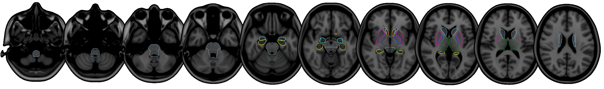
The structural T1w scan in the A2CPS neuroimaging protocol is the source of several pre-specified biomarkers. Two of these biomarkers–the volumes of the hippocampi and amygdalae–are derived from a tool in the Functional Magnetic Resonance Imaging of the Brain (FMRIB) Software Library (FSL): FMRIB’s Integrated Registration and Segmentation Tool (FIRST). The A2CPS pipeline calls FIRST as a part of FSL standard pipeline for processing anatomical images (fsl_anat), which generates several outputs in addition to the biomarkers. This kit provides and overview of the outputs available from that pipeline.

7.1 Starting Project

7.1.1 Locate data

In the release, data are stored underneath the mris/derivatives folder:

/corral-secure/projects/A2CPS/products/consortium-data/pre-surgery/mris/derivatives/fslanat

This folder contains all of the outputs for every participant, with subject folders of the form sub-[recordid]_ses-[protocolid]_T1w.anat. Detailed descriptions of the outputs are available in the fsl_anat documentation.

Many users will not need the raw fsl_anat outputs and can instead rely a table in which the subcortical measures have been aggregated: fslanat.tsv. A data dictionary for this table is available in the fslanat.json file, and also online.

7.1.2 Extract data

In this kit, we will compare volumetric measurements that are produced by both FIRST and FreeSurfer (Chapter 9). In some circumstances, the volumes are largely interchangeable, but for some structures these tools are known to produce fairly different estimates of volume (Sadil & Lindquist, 2024). Let’s replicate part of that analysis.

Sadil, P., & Lindquist, M. A. (2024). Comparing automated subcortical volume estimation methods; amygdala volumes estimated by FSL and FreeSurfer have poor consistency. In Human Brain Mapping (No. 17; Vol. 45, p. e70027). https://doi.org/10.1002/hbm.70027

library(readr)
library(dplyr)
library(tidyr)
library(ggplot2)
library(stringr)
library(purrr)
library(irr)
library(agree)

First, load in the cortical volumes provided by FSL.

fslanat <- read_tsv("data/fslanat/fslanat.tsv", show_col_types = FALSE)
head(fslanat)

Brain-Stem /4th Ventricle	Left-Accumbens-area	Left-Amygdala	Left-Caudate	Left-Hippocampus	Left-Pallidum	Left-Putamen	Left-Thalamus-Proper	Right-Accumbens-area	Right-Amygdala	Right-Caudate	Right-Hippocampus	Right-Pallidum	Right-Putamen	Right-Thalamus-Proper	t1_to_mni_scaling	t1_space_orig_volume	t1_space_mni_volume	sub	ses
24714	582	1696	3631	3213	2040	4107	8117	426	1132	3634	3206	2016	4174	7751	0.514789	1051418	541258.4	20034	V1
20177	497	1472	3309	3951	1681	4385	7400	365	1134	3305	3873	1746	4067	7390	0.515193	1030126	530713.7	10767	V1
22711	609	1645	2822	4529	1705	4857	7520	308	1300	2876	4219	1598	4128	7253	0.710936	1015779	722153.9	20275	V1
21246	394	1164	2863	2414	1620	4274	7011	409	1320	2833	3356	1561	3795	6830	0.968790	944113	914647.2	10292	V1
24811	625	1366	3152	3429	1967	4824	8532	517	1545	3083	3569	1833	4551	7725	0.544569	1142600	622224.5	10826	V1
24092	676	1616	2897	4227	1878	4573	9116	553	1416	3080	4447	1903	4665	9040	1.228005	1224947	1504241.0	20104	V1

In addition to subcortical volumetric information, that table contains a few fields related to the overall size of the brain (t1_to_mni_scaling, t1_space_orig_volume, t1_space_mni_volume). Drop those fields. To make it easier to join with FreeSurfer values, we’ll also unpivot the table into a wider format, and extract information about the hemisphere.

subcort_fsl <- fslanat |>
  select(-starts_with("t1_")) |>
  pivot_longer(-c(sub, ses), values_to = "volume", names_to = "structure") |>
  separate(structure, c("hemisphere", "structure"), sep = "-")

head(subcort_fsl)

sub	ses	hemisphere	structure	volume
20034	V1	Brain	Stem /4th Ventricle	24714
20034	V1	Left	Accumbens	582
20034	V1	Left	Amygdala	1696
20034	V1	Left	Caudate	3631
20034	V1	Left	Hippocampus	3213
20034	V1	Left	Pallidum	2040

Now, grab the equivalent information from FreeSurfer.

subcort_freesurfer <- read_tsv(
  "data/freesurfer/aseg.tsv",
  show_col_types = FALSE
) |>
  filter(str_detect(
    StructName,
    "Thalamus|Putamen|Pallidum|Hippocampus|Amygdala|Accumbens"
  )) |>
  separate(StructName, into = c("hemisphere", "structure"), sep = "-") |>
  select(volume = Volume_mm3, hemisphere, structure, sub, ses)

The tables may now be combined. Note that, while combining them, we add an additional column to keep track of which method produced the volume.

subcort <- bind_rows(
  list(fsl = subcort_fsl, freesurfer = subcort_freesurfer),
  .id = "method"
) |>
  pivot_wider(names_from = method, values_from = volume) |>
  na.omit() # not every structure is available in both methods, and not every participant has been processed by both pipelines


# check which structures we have available
subcort |> distinct(structure)

structure
Accumbens
Amygdala
Hippocampus
Pallidum
Putamen
Thalamus

To compare the structures, make a simple Bland-Altman plot.

Figure 7.1: Comparison of Subcortical Volumes as Estimated by FSL and FreeSurfer. Each dot corresponds to a single structure of a single participant. The blue lines span the 95% confidence interval around the difference of the two estimates of volume, and the red lines are confidence intervals around the limits of agreement.

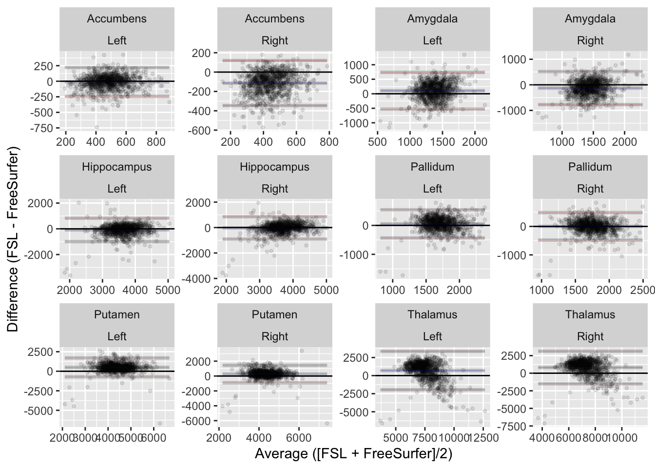
As expected, there are overal differences in how the estimates provided by the two structures Figure 7.1. We can quantify these differences using the intraclass correlation coefficient.

Table 7.1: Consistency of Subcortical Volumes. The lower and upper bounds are 95% Confidence intervals, and the estimate is for the intraclass correlation. By the conventions of McGraw & Wong (1996), this is also known as the \(ICC(C,1)\).

McGraw, K. O., & Wong, S. P. (1996). Forming inferences about some intraclass correlation coefficients. Psychological Methods, 1(1), 30. https://doi.org/10.1037/1082-989X.1.1.30

subcort |>
  group_nest(hemisphere, structure) |>
  mutate(
    fit = map(
      data,
      ~ icc(
        cbind(.x$fsl, .x$freesurfer),
        model = "twoway",
        type = "consistency",
        unit = "single"
      )
    ),
    estimate = map_dbl(fit, pluck, "value"),
    lower = map_dbl(fit, pluck, "lbound"),
    upper = map_dbl(fit, pluck, "ubound")
  ) |>
  select(-data, -fit) |>
  arrange(structure, hemisphere)

hemisphere	structure	estimate	lower	upper
Left	Accumbens	0.5545339	0.5099570	0.5961404
Right	Accumbens	0.4525440	0.4016893	0.5006163
Left	Amygdala	0.1712640	0.1102848	0.2309586
Right	Amygdala	0.2097839	0.1495811	0.2684369
Left	Hippocampus	0.5341598	0.4882153	0.5771516
Right	Hippocampus	0.5844969	0.5420350	0.6239818
Left	Pallidum	0.4685240	0.4185594	0.5156609
Right	Pallidum	0.4980915	0.4498653	0.5434214
Left	Putamen	0.5330968	0.4870825	0.5761597
Right	Putamen	0.5511217	0.5063117	0.5929634
Left	Thalamus	0.3977454	0.3440988	0.4488036
Right	Thalamus	0.4593056	0.4088233	0.5069856

7.2 Considerations While Working on Projects

7.2.1 Variability Across Scanners

Many MRI biomarkers exhibit variability across the scanners, which may confound some analyses. For an up-to-date assessment of the issue and overview of current thinking, please see Confluence.

7.2.2 Data Quality

As with any MRI derivative, all pipeline derivatives have been included. This means that products were included regardless of their quality, and so some products may have been generated from images that are known to have poor quality—rated “red”, or incomparable. For details on the ratings and how to exclude them, see Appendix A. Additionally, extensive QC has not yet been performed on the derivatives themselves, and so there may be cases where pipelines produced atypical outputs. For an overview of planned checks, see Confluence.

7.2.3 Methods

For a subset of participants, the standard fsl_anat pipeline needed to be modified.

7.2.3.1 Field-of-View Estimation in UC

An early step in this pipeline involves estimating the field-of-view and cropping the image to a standard size. The cropping is done with the FSL tool robustfov, which uses a heuristic to first identify the most superior slice that could include the skull, uses a pre-specified distance in mm to select an inferior slice that is expected to be below the cerebellum, and crops everything outside of those slices. The heuristic is based on the quantiles of intensity values, but this heuristic was observed to often fail for data collected with SENSE.

To accommodate scans that failed for this reason, a small amount of noise was added to the entire image, and then the field-of-view was estimated on this degraded image. The field-of-view was then applied to the original image, and that cropped image was provided to fsl_anat (with automated cropping disabled). This workaround was recommended by Mark Jenkinson on the FSL Archives, and it was applied to these subjects.

7.2.3.2 High-Intensity Voxels

A subset of cases exhibited poor alignment to the standard space, with the misalignment driven by high-intensity voxels from outside of the brain. The extreme intensity values may have been driven by relatively high proportions of fatty tissue. For cases where these failures were identified, a mask was generated from the top 1% of voxels, which was then visually inspected to confirm that it did not include any voxels in the brain. That mask was then provided to fsl_anat as a “lesion” mask (via a hidden option), resulting in those voxels being ignored during alignment. In instances where the mask included brain voxels, the fsl_anat results were not included. The list of participants this fix was applied to is here.

7.2.4 Citations

The fsl_anat pipeline relies on several tools that are the products of research by the FMRIB team. If you use these derivatives in your analyses, please follow the instructions for citations here: https://fsl.fmrib.ox.ac.uk/fsl/docs/index.html.

In publications or presentations including data from A2CPS, please include the following statement as attribution:

Data were provided [in part] by the A2CPS Consortium funded by the National Institutes of Health (NIH) Common Fund, which is managed by the Office of the Director (OD)/ Office of Strategic Coordination (OSC). Consortium components and their associated funding sources include Clinical Coordinating Center (U24NS112873), Data Integration and Resource Center (U54DA049110), Omics Data Generation Centers (U54DA049116, U54DA049115, U54DA049113), Multi-site Clinical Center 1 (MCC1) (UM1NS112874), and Multi-site Clinical Center 2 (MCC2) (UM1NS118922).

Note

The following published papers should be cited when referring to A2CPS Protocol and Biomarkers: Sluka et al. (2023) Berardi et al. (2022)

Berardi, G., Frey-Law, L., Sluka, K. A., Bayman, E. O., Coffey, C. S., Ecklund, D., Vance, C. G. T., Dailey, D. L., Burns, J., Buvanendran, A., McCarthy, R. J., Jacobs, J., Zhou, X. J., Wixson, R., Balach, T., Brummett, C. M., Clauw, D., Colquhoun, D., Harte, S. E., … Wandner, L. D. (2022). Multi-site observational study to assess biomarkers for susceptibility or resilience to chronic pain: The acute to chronic pain signatures (A2CPS) study protocol. Frontiers in Medicine, 9. https://doi.org/10.3389/fmed.2022.849214

Sluka, K. A., Wager, T. D., Sutherland, S. P., Labosky, P. A., Balach, T., Bayman, E. O., Berardi, G., Brummett, C. M., Burns, J., Buvanendran, A., et al. (2023). Predicting chronic postsurgical pain: Current evidence and a novel program to develop predictive biomarker signatures. Pain, 164(9), 1912–1926. https://doi.org/10.1097/j.pain.0000000000002938

Sadil, P., Arfanakis, K., Bhuiyan, E. H., Caffo, B., Calhoun, V. D., Clauw, D. J., DeLano, M. C., Ford, J. C., Gattu, R., Guo, X., Harris, R. E., Ichesco, E., Johnson, M. A., Jung, H., Kahn, A. B., Kaplan, C. M., Leloudas, N., Lindquist, M. A., Luo, Q., … Chronic Pain Signatures Consortium, T. A. to. (2024). Image processing in the acute to chronic pain signatures (A2CPS) project. bioRxiv. https://doi.org/10.1101/2024.12.19.627509

When using neuroimaging derivatives, please also cite Sadil et al. (2024).